
Explaining Adversarial Examples by Local Properties of Convolutional
Neural Networks
Hamed H. Aghdam, Elnaz J. Heravi and Domenec Puig
Computer Engineering and Mathematics Department, Rovira i Virgili University, Tarragona, Spain
{hamed.habibi, elnaz.jahani, domenec.puig}@urv.cat
Keywords:
Adversarial Examples, Convolutional Neural Networks, Lipschitz Constant.
Abstract:
Vulnerability of ConvNets to adversarial examples have been mainly studied by devising a solution for gen-
erating adversarial examples. Early studies suggested that sensitivity of ConvNets to adversarial examples
are due to their non-linearity. Most recent studies explained that instability of ConvNet to these examples are
because of their linear nature. In this work, we analyze some of local properties of ConvNets that are directly
related to their unreliability to adversarial examples. We shows that ConvNets are not locally isotropic and
symmetric. Also, we show that Mantel score of distance matrices in the input and output of a ConvNet is very
low showing that topology of points located at a very close distance to a samples might significantly change
by ConvNets. We also explain that non-linearity of topology changes in ConvNet are because they apply an
affine transformation in each layer. Furthermore, we explain that despite the fact that global Lipschitz constant
of a ConvNet might be greater than 1, it is locally less than 1 in most of adversarial examples.
1 INTRODUCTION
Despite their success in various tasks of computer
vision, Convolutional Neural Networks (ConvNets)
suffer from sensitivity to adversarial examples. In
general, an adversarial example is an example which
is generated by slightly perturbing the original sam-
ple. Sensitivity of ConvNets to adversarial samples
was first discovered by (Szegedy et al., 2014b). Re-
searchers further studies adversarial samples by creat-
ing perturbation vectors using various objective func-
tions. Recently, (Goodfellow et al., 2015) suggested
that vulnerability of ConvNets to adversarial samples
is due to their linear nature.
To our knowledge, previous works have not ana-
lyzed local properties of ConvNets that are directly re-
lated to their stability against adversarial examples. In
this paper, we study some of these properties in order
to better explain the reason that ConvNets might be
sensitive to small perturbations. Specifically, we con-
duct various data-driven studies and show that Con-
vNets are likely not to be isotropic and symmetric
around original samples. We support these hypoth-
esis by analyzing the convolution operation in the fre-
quency domain and showing that permutation of in-
put can change the output of the convolution. For this
reason, a ConvNet might compute different scores for
two adversarial examples located at the same distance
from original sample. In addition, we explain why a
ConvNet might not be isotropic. Besides, we show
that although adversarial examples are very close to
the original sample it is highly probable that their
topology changes greatly by ConvNets. This behavior
is also explained in terms of affine transformation and
distance matrices. Our empirical Lipschitz analysis
reveals that the global Lipschitz constant can be high
(greater than 1) but it is usually less than 1 when we
study the Lipschitz constant in a small region around
each clean sample.
2 EMPIRICAL STUDY
In general, an adversarial example x
a
is defined as:
x
a
= x + ν (1)
where ν ∈ [−ε, ε]
H×W ×3
is the perturbation vector and
x ∈ R
H×W ×3
is the original image. Representing the
classification score of a ConvNet by Φ : R
H×W ×3
→
[0, 1]
K
, we can find ν using two different approaches
including optimization-based and data-driven. Given
the original image x and its actual class label k, the
former approaches try to minimize a regularized ob-
jective function. The objective function can be min-
imizing the score of the actual class regularized by
226
Aghdam H., Heravi E. and Puig D.
Explaining Adversarial Examples by Local Properties of Convolutional Neural Networks.
DOI: 10.5220/0006123702260234
In Proceedings of the 12th International Joint Conference on Computer Vision, Imaging and Computer Graphics Theory and Applications (VISIGRAPP 2017), pages 226-234
ISBN: 978-989-758-226-4
Copyright
c
2017 by SCITEPRESS – Science and Technology Publications, Lda. All rights reserved

|
ν
|
in order to find perturbations which are not eas-
ily perceivable to human eye (Szegedy et al., 2014b).
(Aghdam et al., 2016) also proposed another objec-
tive function to find ν such that x
a
is misclassified but
its distance from decision boundary is minimum.
In contrast, the latter approach finds ν by gen-
erating many candidates which satisfy the condition
|
ν
|
≤ T where T is a threshold value. (Goodfellow
et al., 2015) compute sign(∇Φ(x)) and generate x
a
by
setting ν = εsign(∇Φ(x )) and applying a line search
over ε. The optimization-based approaches help us
to quickly study stability of a ConvNet to small per-
turbations. However, they do not provide detailed
information about adversarial samples and response
of ConvNets to small perturbations. Besides, dis-
tribution of the values in the perturbation vector ν
found by these techniques may not follow a specific
distribution. Moreover, the data-driven technique in
(Goodfellow et al., 2015) is mainly used for regu-
larizing a ConvNet and it has the same issues as the
optimization-based techniques.
In this work, we have conducted a data-
driven technique for studying local properties of
ConvNets. Specifically, we are mainly inter-
ested in properties which are related to stabil-
ity of ConvNets against small perturbations. We
study these properties on AlexNet(Krizhevsky et al.,
2012), GoogleNet(Szegedy et al., 2014a), VGG
Net(Simonyan and Zisserman, 2015), Residual
Net(He et al., 2015) trained on ImageNet dataset as
well as the ConvNets in (Ciresan et al., 2012) and
(Aghdam et al., 2015) trained on the German Traffic
Sign Benchmark (GTSRB) dataset(?).
2.1 Isotropic
A zero-centered function is isotropic if it returns an
identical value for all points located at specific dis-
tance from origin. We say Φ(x ) is locally isotropic at
point a ∈ R
W
× H × 3 if:
∀
ν
1
,ν
2
∈[−ε,ε]
W ×H×3
∧kν
1
k=kν
2
k=R
Φ(a +ν
1
) = Φ(a + ν
2
) (2)
where ν
1
and ν
2
are the perturbations vectors and a
is the original image. In other words, the output of
the function at all points located at distance R from a
must be identical. Mathematically speaking, we can
approximate Φ(x
a
) using the Taylor theorem. For-
mally:
Φ(x
a
) = Φ(x +ν) = Φ(x) +∇Φ(x)ν +
1
2
ν
T
H(Φ(x))ν (3)
where ∇ and H(.) are the gradient and Hessian of
Φ(x). Based on this equation, a ConvNet is locally
isotropic at x if elements of ∇ are identical and H(.)
is a diagonal matrix where the non-zero elements are
equal. Therefore, isotropic property can be measured
during backpropagation by computing the pairwise
difference between elements of ∇Φ(x). However, re-
sults obtained by this way might not be promising.
This is due to the fact that (3) approximates the out-
put using only the first and second gradients. Theo-
retically, if Φ(x) is flat near x
a
both ∇ and H(.) will
be zero showing that Φ(x) is isotropic in a very small
region close to x.
To analyze a larger region around x, we need
higher order terms in (3). Since approximating us-
ing higher order terms is not trivial in (3), we analyze
isotropic property of different ConvNets empirically.
To be more specific, given original image x, we com-
pute:
∀
r∈[ε,1,...,R]
∀
i∈{1,...,T }
s
r
i
= Φ(x + r
ν
i
kν
r
i
k
)
s.t. ν
r
i
= U(−1, 1).
(4)
In this equation, U indicates the uniform distribution.
According to this equation, we generate T perturba-
tions that all of them are located at distance r from
x and compute the classification score of x
a
. We set
T = 100 and R = 20 and computed the above equation
on 300 samples for each ConvNet and its correspond-
ing dataset. It is worth mentioning that we pick the
samples that are classified correctly by ConvNet with
more than 99% confidence. Figure 1 illustrates the
results.
The horizontal axe shows the radius and the
vertical axe shows the range of score (in logarith-
mic scale) for each radius and each sample ob-
tained by computing range(r) = max(∀
i∈{1,...,T }
s
r
i
) −
min(∀
i∈{1,...,T }
s
r
i
). Ideally, if Φ(x) is isotropic around
x, range(r) must be zero for all adversarial examples
located at distance r from x. In addition, color of each
circle in this figure shows the mean score of the ad-
versarial samples. Finally, square markers shows that
there was at least one adversarial example at that par-
ticular radius that has been misclassifed by the Con-
vNet.
We observe that none of the ConvNets are per-
fectly isotropic even at distance ε from a sample.
However, their score does not significantly change at
distance ε. By increasing the radius to 1 pixel, all
ConvNets become more non-isotropic. Finally most
of ConvNets become very non-isotropic at distance
10 pixels.
2.2 Symmetricity
Mathematically, multivariate function f (X) =
f (x
1
, . . . , x
n
) is symmetric if its value for any permu-
tation of input arguments is identical. For instance,
Explaining Adversarial Examples by Local Properties of Convolutional Neural Networks
227

Figure 1: Isotropic property of different ConvNets. Refer to text for detailed information.
f (x
1
, x
2
) is symmetric if f (a
1
, a
2
) = f (a
2
, a
1
) for
all values of a
1
and a
2
. Also, f (x
1
, . . . , x
n
) is locally
symmetric at point [a
1
, . . . , a
2
] if
f (a + ν), [ν
1
, ν
2
, . . . , ν
n
] ∈ [−ε, ε]
n
(5)
is identical for all permutations of perturbation vector
ν. In terms of images and a ConvNet, Φ(x
a
) must be
identical for all permutations of ν.
This means that re-ordering the elements of ν
must not change the output. This property is de-
scribed on Figure 2. The background shows the value
of Φ(x) in the region nearby the illustrated image in
this figure. It is clear that Φ(x) is maximum given
the clean image x. Assume two perturbation vectors
ν
1
and ν
2
where ν
2
is obtained by re-ordering the ele-
ments of ν
1
. It is expected that Φ(x+ν
1
) = Φ(x+ν
2
)
since probability density function of elements of ν
1
and ν
2
are identical and kν
1
k = kν
2
k = ε. Note that
the perturbation vectors are not perceivable on the
perturbed images to human eye in this figure. Fur-
thermore, Φ(x) is not symmetric at the given image
in this figure. Hence, one of them is classified as
another class since it falls into a region where the
classification score is low. Notwithstanding, if Φ(x)
was symmetrical at the given image both perturbed
images would be classified correctly. Consequently,
symmetricity is an important property for being toler-
ant against small perturbations.
Note that an isotropic function is also symmetric.
In addition, if a function is not isotropic, it is still pos-
sible that the function possess the symmetrical prop-
erty. To empirically study local symmetricity of Φ(x),
we performed the following procedure on each sam-
ple in dataset:
∀
r∈[ε,R]
∀
i∈{1,...,T }
s
r
i
= Φ(x + permute(r
ν
r
kν
r
k
))
s.t. ν
r
= U(−1, 1).
(6)
Configuration of the parameters in this equation is
VISAPP 2017 - International Conference on Computer Vision Theory and Applications
228

Figure 2: ConvNets must be symmetry at x.
similar to Section 2.1. Figure 3 shows the results on
different ConvNets. The results suggest that except
for adversarial example in distance less than ε from x,
none of the ConvNets are symmetric.
We argue that being locally isotropic is an impor-
tant property for having a more tolerant ConvNet to
adversarial examples. To be more specific, we ex-
pect that all adversarial samples that are located at
the same distance from the original samples to have
identical scores. Radial Basis Function networks in-
trinsically possess this property since features that are
located in an equal distance from the basis canters will
have identical values. However, feature extraction in
ConvNets is mainly based on convolution operations.
Assume a convolution kernel K = [k
i j
] ∈ R
Q×P
and
two different adversarial examples x
1
a
, x
2
a
∈ [−ε, ε]
H×W
where kx
1
a
k = ε and x
2
a
= permute(x
1
a
). Denoting the
convolution operation by ∗, it is provable that K ∗x
1
a
6=
K ∗ x
2
a
if ∃
i j
k
i
> 0 ∧ k
j
> 0. To verify this, we study
the convolution operation in the frequency domain.
Convolution in spatial domain equals to multiplica-
tion in frequency domain. In other words, K ∗ x
1
a
=
F (K).F(x
1
a
) and K ∗ x
2
a
= F (K).F(x
2
a
) where F (.)
transforms the input into frequency domain. The term
K ∗ x
1
a
will be equal to K ∗ x
2
a
if F(x
1
a
) = F(x
2
a
). Since
x
1
a
and x
2
a
are two different inputs, their Fourier trans-
form will not be identical. Then, F(x
1
a
) 6= F(x
2
a
) which
shows that convolving the same filter with permuted
inputs does not produce identical results. Notwith-
standing, if kx
1
a
k is close to zero, the results of convo-
lution operation becomes more comparable.
Extending this fact to ConvNets, we realize that
output of the first convolution layer in a ConvNet will
not be similar (except very few cases such as setting
values of all weights to zero) given two inputs x
1
a
and
x
2
a
where x
2
a
= permute(x
1
a
). Then, the output of the
first layer may pass through a MAX-pooling layer
where the outputs become more dissimilar. This is
one explanation that why ConvNets in Figure 1 and
Figure 3 are not isotropic and symmetrical.
Based on (3), one may argue that we can add reg-
ularization terms to the objective function in order
to minimize the norm of gradient vector and Hessian
matrices at each training sample. However, it should
be noted that, this can make a function isotropic and
symmetric in a very small region since we do not take
into account higher order derivatives. Results in Fig-
ure 1 and Figure 3 shows that ConvNets are reason-
ably locally isotropic in very small region. As the re-
sult, regularizing by the aforementioned terms might
not improve the stability significantly.
2.3 Topology Preservation
From one point of view, a ConvNet transforms a
D
input
dimensional input vector to a D
out put
dimen-
sional vector in the layer just before the classification
layer. For example, AlexNet transforms a 256×256×
3 dimensional vector to a 4096 dimensional vector in
layer fc2.
Assume X
input
= {X
1
input
, . . . , X
N
input
} is a set of
D
input
dimensional vectors each representing raw
pixel intensities. Also, considering that Φ
L
(X) :
R
D
input
→ R
D
out put
is the output of the L
th
layer
in a ConvNet, Φ
L
(X
input
) returns set X
out put
=
{X
1
out put
, . . . , X
N
out put
} where each element is obtained
by applying Φ
L
(x) on the corresponding element in
X
input
.
By defining a metric such as Euclidean distance,
we can view X
input
and X
out put
as two different topo-
logical spaces. While the topology of points in X
input
is not suitable for the task of classification, topology
of points in X
out put
has been adjusted such that the
classes become linearly separable in this space. It is
clear that topology of these two spaces are likely to be
very different.
Now, assume set x
perturbed
input
= {x + ν
1
, . . . , x +
ν
N
} including perturbed examples of x where ν
i
∈
[−ε, −ε]
D
input
. While it is clear that topology of scat-
tered points in X
input
changes greatly using Φ
L
(X)
(because classification accuracy of raw points in
X
input
is usually much lower that points in X
out put
),
we are not sure how Φ
L
(X) affects the topology of
points in x
perturbed
. Note that points in x
perturbed
input
are
very close together before applying Φ
L
(X) on them.
Lets assume the simplest scenario where Φ
L
(X) =
XW and W ∈ R
D
input
×D
out put
is a weight matrix. In
other words, we assumed that Φ
L
(X) transforms the
points to a new space by using a linear transfor-
mation. One way to show topology of X
input
and
X
out put
is to compute a distinct distance matrix for
each of them where element i j in this matrix is ob-
tained by computing kX
i
− X
j
k = kd
i j
k = d
i j
d
T
i j
. As-
suming Φ
L
(X) = XW , the element i j in distance ma-
trix of the transformed space will equal to kX
i
W −
X
j
W k = |k(X
i
− X
j
)W k = kd
i j
W k = d
i j
W (d
i j
W )
T
.
Explaining Adversarial Examples by Local Properties of Convolutional Neural Networks
229
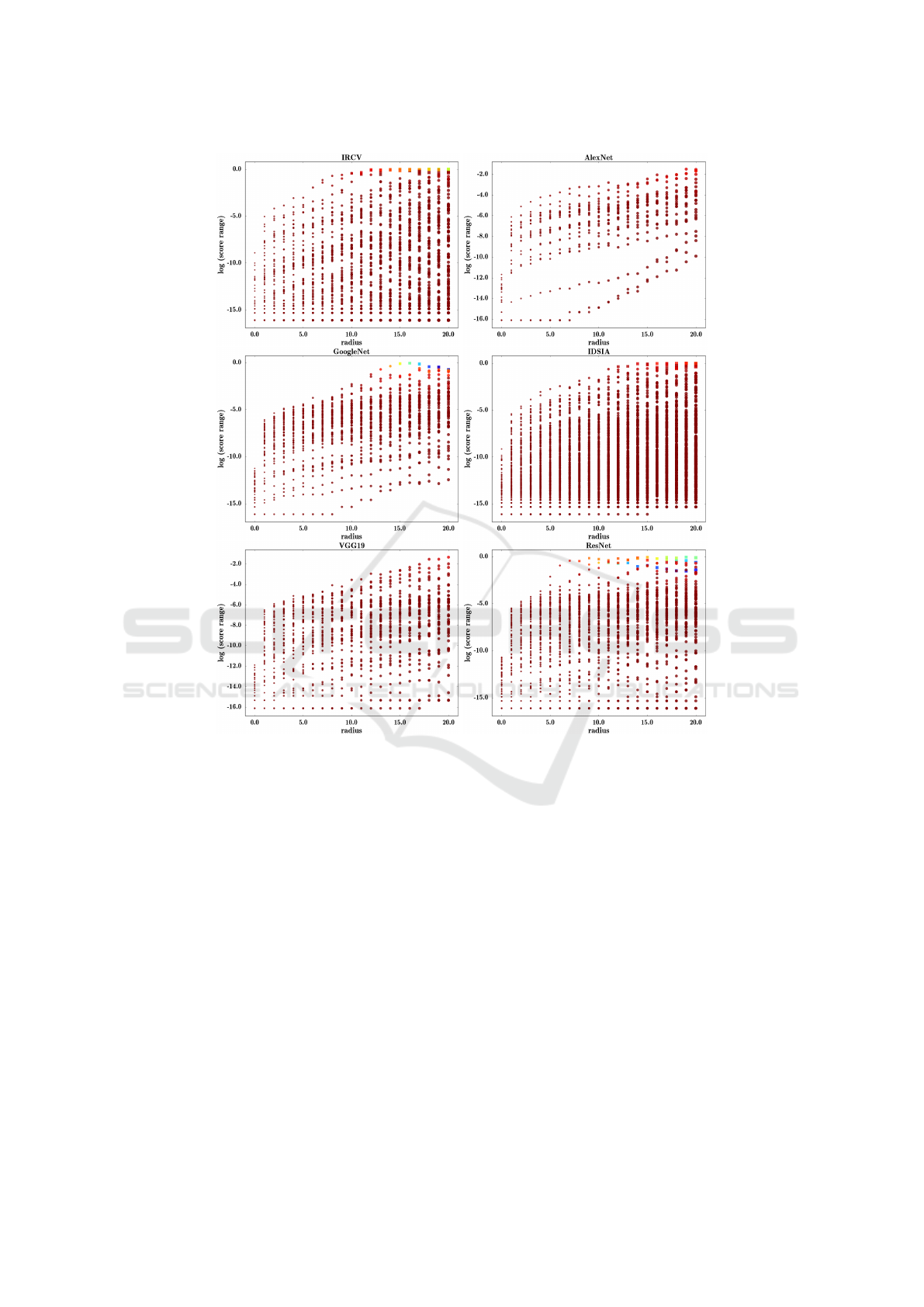
Figure 3: Symmetricity property of different ConvNets. Refer to text for detailed information.
Using the properties of matrix transpose, we obtain
d
i j
W (d
i j
W )
T
= d
i j
WW
T
d
T
i j
. This means that the re-
lation between distance matrix of X
input
and distance
matrix of X
out put
is not necessarily linear even when
Φ
L
(X) is a linear function. We say a transforma-
tion preserves the topology of X
input
when the dis-
tances matrix of X
out put
is a linear function of distance
matrix of X
input
. For example scaling a set of two
dimensional vectors does not change their topology
since the distance matrix of the transformed points is
a scaled version of the distance matrix of the origi-
nal points. But, applying an affine transformation on
them can change their topology.
Changing topology means that the distances be-
tween different points are manipulated nonlinearly.
In other words, if the closest point to A is point
C in the original space, the closest point to A
might be point B in the transformed space. Our
aim is to determine how a ConvNet affects topol-
ogy of points in x
perturbed
input
. Denoting the distance
matrix of x
perturbed
input
with D
input
and distance ma-
trix of x
perturbed
out put
= {Φ
L
(x + ν
1
), . . . , Φ
L
(x + ν
N
)} with
D
out put
, we can compute:
α = D
−1
input
D
out put
. (7)
If applying Φ
L
(X) does not change the topology of
x
perturbed
input
, matrix α ∈ R
N×N
will be diagonal with
identical values. Even though α tells us how topol-
ogy of points exactly changes after applying Φ
L
(X)
but it is not trivial to compute a score using α repre-
senting degree of non-linearity of topology changes.
For this reason, we utilized Mantel test for compar-
ing two distance matrices. Specifically, Mantel test
compute the Pearson product-moment correlation co-
efficient ρ using many permutations of element of dis-
tance matrices. We say the relation between two ma-
trices is linear when |ρ| = 1. To empirically study
VISAPP 2017 - International Conference on Computer Vision Theory and Applications
230

this property of ConvNets we followed the procedure
in (4) to generate adversarial examples in specific
radii. Then, we computed the Mantel score between
x
perturbed
input
and x
perturbed
out put
for each ConvNet separately.
Figure 4 shows the results.
We observe that topology of point does not lin-
early change even when they are very close to x. This
is due to the fact that the Mantel score for all of Con-
vNets is −0.1 < ρ < 0.1. As we mentioned earlier,
a simple linear transformation such as affine transfor-
mation changes the topology of points. If we think
of ConvNets as fully-connected networks with shared
weights, we realize that every neuron in this network
applies the affine transformation f (XW + b) on its in-
puts where f (.) is an activation function. This affine
transformation changes the topology of points. Con-
sidering a deep network with several convolution lay-
ers, the input passes through multiple affine transfor-
mations which greatly changes the topology of inputs.
As the result, points located at distance ε from the
original sample will not have the same topology at
the output of a ConvNet.
2.4 Lipschitz
The method discussed in Section 2.3 takes into ac-
count all pair-wise distances between samples in or-
der to compare topology of points before and after
applying Φ
L
(X). Lipschitz analysis is an alternative
method to study non-linearity of a function. Specif-
ically, given X
1
, X
2
∈ R
D
input
and function Φ
L
(X) :
R
D
input
→ R
D
out put
, Lipschitz analysis finds a constant
L called Lipschitz constant such that:
kΦ
L
(X
1
) − Φ
L
(X
2
)k ≤ LkX
1
− X
2
k
f or all X
1
, X
2
∈ R
D
input
.
(8)
This definition studies the global non-linearity of a
function. Szegedy et.al. (Szegedy et al., 2014b)
showed how to compute L for a ConvNet with convo-
lution, pooling and activation layers. Notwithstand-
ing, Lipschitz constant L found by applying (8) on
whole domain of a ConvNet does not accurately tell
us how output of the ConvNet changes locally. This
problem is shown in Figure 5. We see that the pur-
ple function is more non-linear than the yellow func-
tion. This is due to the fact that its non-linearity is
less when |x| > 5. Notwithstanding, degree of non-
linearity of both function are similar when −5 < x <
5. The Lipschitz analysis in (8) does not take into
account local non-linearity of a function. Instead, it
find L which equals to greatest gradient magnitude in
whole domain of the function.
Our aim is to study behaviour of function on ad-
versarial examples. Therefore, we must compute Lip-
schitz constant L locally. To be more specific, denot-
ing an adversarial sample with x
a
= x + ν and a clean
sample with x we find L
x
such that:
kg(Φ
L
(x
a
)) − g(Φ
L
(x))k ≤ L
x
kh(x
a
) − h(x)k
f or all ν ∈ [−ε, ε]
D
input
.
(9)
where g(.) and h(.) are two function to normalize
their input. From topology point of view, the above
equation studies how adversarial examples are trans-
formed by a ConvNet with respect to the original sam-
ple. If L
x
< 1 for all adversarial samples, this means
that Φ
L
(X) attracts the adversarial examples toward
the clean sample (They become closer to the clean
sample after being transformed to D
out put
dimensional
space by the ConvNet). However, the distance be-
tween adversarial examples and the clean example re-
mains unchanged when L
x
= 1 for all adversarial sam-
ples. Finally, Φ
L
(X) repels the adversarial examples
from the clean sample when L
x
> 1.
A ConvNet will be more tolerant against adver-
sarial samples when L
x
< 1. This is due to the fact
that when adversarial samples get closer to the clean
sample, it is more likely that they have classification
scores close to the clean sample. To empirically study
the Lipschitz constant, we generated the samples us-
ing (4) and computed kΦ
L
(x + ν) − Φ
L
(x)k as well
as kνk. It is worth mentioning that the clean samples
as well as ν
r
i
in (4) are the same for all the ConvNets
trained on the same dataset. In addition, g() and h()
are two separate min-max normalizers in which their
parameters are obtained by feeding thousands of sam-
ples to each ConvNet and collecting the minimum and
maximum value in the input and output of the Con-
vNet. Finally, each sample has a unique seed for the
uniform noise function. This means that if we run the
algorithm many times on different ConvNets for the
sample i, the same adversarial examples will be gener-
ated in all the cases. By this way, we can compare the
results from the ConvNets trained on the same dataset.
Figure 6 shows the relation between these two fac-
tors. In addition, the black and blue lines are obtained
by fitting a first order (linear regression) and second
order polynomial on data. Color of each point corre-
sponds to the radius to which the adversarial sample
is located. The colder color shows a smaller radius.
Even though (Szegedy et al., 2014b) mentioned
that the global Lipschitz constant on AlexNet is
greater than 1, our empirical analysis revealed that all
of the ConvNets in our study are in general locally
contraction. In other words, the Lipschitz constant
on is less than 1 in most of the cases meaning that
adversarial examples become closer to the original
sample despite the fact that their topology changes by
Φ
L
(x). This suggests that that although ConvNet are
Explaining Adversarial Examples by Local Properties of Convolutional Neural Networks
231
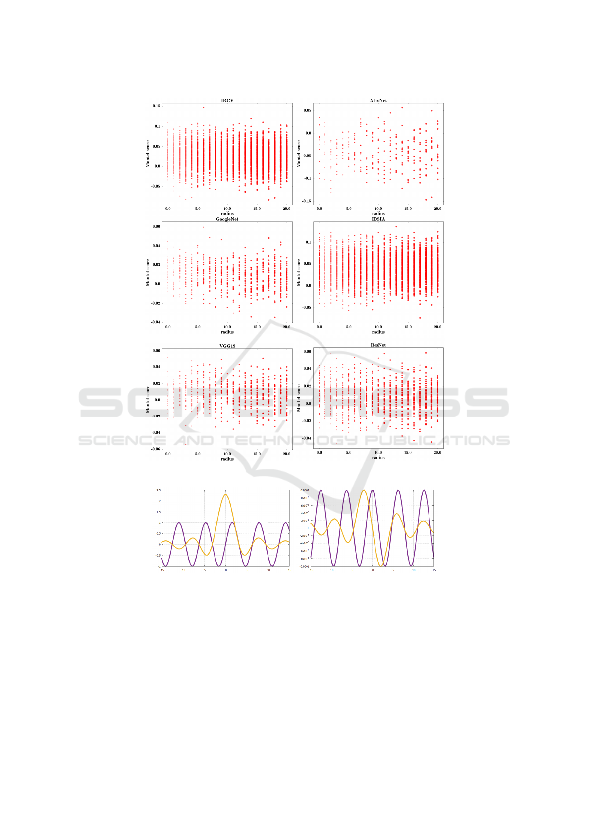
Figure 4: Topology preservation in ConvNets. Refer to text for detailed information.
Figure 5: Two functions with identical Lipschitz constants. Left) Plot of two functions and Right) Derivative of two functions.
non-linear functions, they are generally locally con-
traction. As the result, explaining adversarial exam-
ples with global properties related to non-linearity of
ConvNet might not be accurate.
3 CONCLUSION
In this paper, we empirically studied local proper-
ties of various ConvNets that are related to their vul-
nerability to adversarial examples. Specifically, we
showed that state-of-art ConvNets trained on Ima-
geNet and GTSRB datasets are not isotropic and sym-
metric around original samples. This means when we
add two noise vectors with identical magnitudes to the
clean sample, classification score of the adversarial
examples might not be similar. We explained the rea-
son in frequency domain. In addition, we studied how
topology of adversarial examples located around the
clean samples are affected by the ConvNet. We found
VISAPP 2017 - International Conference on Computer Vision Theory and Applications
232

Figure 6: Topology preservation in ConvNets. Refer to text for detailed information.
that ConvNets change the topology of adversarial ex-
amples even when they are very close to clean sam-
ples. Finally, we analyzed the distance of adversarial
examples in the input domain and the output of Con-
vNets. We found that adversarial examples are very
likely to become closer to clean samples after being
transformed by a ConvNet to a new space.
ACKNOWLEDGEMENTS
Hamed H. Aghdam and Elnaz J. Heravi are grateful
for the supports granted by Generalitat de Catalunya’s
Ag
`
ecia de Gesti
´
o d’Ajuts Universitaris i de Recerca
(AGAUR) through the FI-DGR 2015 fellowship and
University Rovira i Virgili through the Marti Franques
fellowship, respectively.
REFERENCES
Aghdam, H. H., Heravi, E. J., and Puig, D. (2015). Rec-
ognizing Traffic Signs using a Practical Deep Neural
Network. In Robot 2015: Second Iberian Robotics
Conference, pages 399–410, Lisbon. Springer.
Aghdam, H. H., Heravi, E. J., and Puig, D. (2016). Ana-
lyzing the Stability of Convolutional Neural Networks
Against Image Degradation. In Proceedings of the
11th International Conference on Computer Vision
Theory and Applications.
Ciresan, D., Meier, U., and Schmidhuber, J. (2012). Multi-
column deep neural networks for image classification.
In 2012 IEEE Conference on Computer Vision and
Pattern Recognition, number February, pages 3642–
3649. IEEE.
Goodfellow, I. J., Shlens, J., and Szegedy, C. (2015). Ex-
plaining and Harnessing Adversarial Examples. Iclr
2015, pages 1–11.
He, K., Zhang, X., Ren, S., and Sun, J. (2015). Deep
Residual Learning for Image Recognition. In arXiv
prepring arXiv:1506.01497.
Krizhevsky, A., Sutskever, I., and Hinton, G. (2012). Im-
agenet classification with deep convolutional neural
networks. In Advances in neural information process-
ing systems, pages 1097–1105. Curran Associates,
Inc.
Simonyan, K. and Zisserman, A. (2015). Very Deep Con-
volutional Networks for Large-Scale Image Recogni-
Explaining Adversarial Examples by Local Properties of Convolutional Neural Networks
233

tion. In International Conference on Learning Repre-
sentation (ICLR), pages 1–13.
Szegedy, C., Reed, S., Sermanet, P., Vanhoucke, V., and
Rabinovich, A. (2014a). Going deeper with convolu-
tions. In arXiv preprint arXiv:1409.4842, pages 1–12.
Szegedy, C., Zaremba, W., and Sutskever, I. (2014b). In-
triguing properties of neural networks.
VISAPP 2017 - International Conference on Computer Vision Theory and Applications
234
