Identification of Types of Corrosion through Electrochemical Noise using
Machine Learning Techniques
Lorraine Marques Alves, Romulo Almeida Cotta and Patrick Marques Ciarelli
Federal University of Espírito Santo, Av. Fernando Ferrari, 514, Vitória-ES, Brazil
Keywords:
Corrosion, Electrochemical Noise, Machine Learning, Wavelet Transform.
Abstract:
Several systems in industries are subject to the effects of corrosion, such as machines, structures and a lot of
equipment. As consequence, the corrosion can damage structures and equipment, causing financial losses and
accidents. Such consequences can be reduced considerably with the use of methods of detection, analysis and
monitoring of corrosion in hazardous areas, which can provide useful information to maintenance planning
and accident prevention. In this paper, we analyze features extracted from electrochemical noise to identify
types of corrosion, and we use machine learning techniques to perform this task. Experimental results show
that the features obtained using wavelet transform are effective to solve this problem, and all the five evaluated
classifiers achieved an average accuracy above 90%.
1 INTRODUCTION
Several very important systems in the industrial field
are subject to the effects of corrosion: means of trans-
portation, such as trains and ships, transmission tow-
ers, storage tanks, heat exchangers and boilers, reac-
tors, etc., causing the deterioration of structures and a
lot of equipment, as well as accidents (Gentil, 2003).
Regarding the losses in the economic sector, corro-
sion can be a source of unplanned costs. The global
cost of corrosion is estimated around U$ 2.5 trillion,
equivalent to 3.4% of world GDP (Gross National
Product) (Koch et al., 2016). Many industries have
realized that the lack of corrosion management can be
very expensive, and that through proper management
of corrosion they can obtain significant cost reduction
(Koch et al., 2016). This factor highlights the impor-
tance of developing research and technology in this
field.
Fortunately, due to the simultaneous occurrence
of oxidation and reduction reactions during the cor-
rosion process, it is possible to measure the current
and electrical potential fluctuations on the surfaces
that are suffering this process. These measured sig-
nals are called electrochemical noise (ECN) (Fofano
and Jambo, 2007).
Some types of corrosion, such as pitting, are
hardly detected using traditional electrochemical
techniques, however, analysis of electrochemical
noise enables its identification and monitoring (Rios
et al., 2013). The identification of corrosion type that
is affecting the metal enables the planning and im-
plementation of more effective solutions for the treat-
ment and prevention in the affected areas. An exam-
ple is the choice of the best inhibitor material, that
can provide greater protection to the metal (Barr et al.,
2001).
This work describes a methodology for the detec-
tion of corrosion types using machine learning tech-
niques and features extracted from electrochemical
noise. Machine learning is a sub-field of artificial
intelligence that is compose by a set of techniques
that are able to learn by examples how a task must
be done. Thus, they are not programmed to do a
task, but they “learn” how to do it. Machine learn-
ing (ML) techniques have been successfully utilized
in various process control, monitoring and optimiza-
tion applications in different industries. Some appli-
cations of ML are: tool for machine condition mon-
itoring, fault diagnosis, image recognition to identify
damaged products, food quality control, classification
of polymers and several other applications (Wuest et
al., 2016). However, few researches to identify types
of corrosion have used this type of approach (Jian
et al., 2013), being this one of the motivations of this
work.
In this paper, techniques that are able to learn by
example are used to detect automatically some dif-
ferent types of localized corrosion, such as pitting,
crevice corrosion and the watermark, as well as the
332
Alves, L., Cotta, R. and Ciarelli, P.
Identification of Types of Corrosion through Electrochemical Noise using Machine Learning Techniques.
DOI: 10.5220/0006122403320340
In Proceedings of the 6th International Conference on Pattern Recognition Applications and Methods (ICPRAM 2017), pages 332-340
ISBN: 978-989-758-222-6
Copyright
c
 2017 by SCITEPRESS – Science and Technology Publications, Lda. All rights reserved

occurrence of passivation on the metal surface, which
is the state in which the behavior of an electrical dou-
ble layer in the solution-electrode interface forms a
protective film that is resistant to corrosion (Fernan-
des et al., 2001). The results obtained in experiments
indicate that the presented approach is promising to
identify some types of localized corrosion, as well as
the occurrence of passivation on metals.
The remainder of this paper is organized as fol-
lows. In Section 2, we present some useful tools
in data analysis of electrochemical noise, including
the wavelet transform. In Section 3, we describe ba-
sic concepts of machine learning and the classifiers
used in the experiments. Subsequently, in Section
4 is shown the materials and methodology used in
the measurements of potential and current of electro-
chemical noise. In Section 5, we present the experi-
ments and achieved results. Our conclusions and sug-
gestions for future work are presented in Section 6.
2 ELECTROCHEMICAL NOISE
DATA ANALYSIS
ECN analysis can be performed so that the potential
and current noise data are processed independently,
using statistical measures, such as mean, standard de-
viation, kurtosis and skewness for the interpretation of
the data. The relationship between the two signals can
also be analyzed using the concept of electrochemical
noise resistance (R
n
), defined as the standard devia-
tion of the potential σ
E
divided by the standard devi-
ation of the current σ
I
, according to equation 1:
R
n
=
σ
E
σ
I
. (1)
The R
n
value is associated with the corrosion rate,
and the higher the resistance value, the smaller the
corrosion rate of the metal. The standard deviation
value of the current reflect the fluctuation magnitude
of the current in the system and, therefore, it can be
used to estimate the corrosion activity (Cottis, 2001).
A methodology for electrochemical noise analy-
sis, called shot noise, considers that the current has
the form of a series of statistically independent charge
packets, and each packet has a short duration of time.
The total charge passing in a certain time interval is
then a sample from a binominal distribution, and if
the average number of pulses is fairly large, it approx-
imates from a normal distribution with known prop-
erties. Applying this theory to electrochemical noise
signals, three parameters can be obtained: average
current of corrosion (I
corr
), average electric charge on
each event (q), and frequency of related events ( f
n
).
These parameters are related by equation 2 (Cottis
and Turgoose, 1999; Cottis, 2001).
I
corr
= q f
n
. (2)
These values cannot be measured directly, but they
can be estimated from the potential and current noise
data, according to equations 3 and 4 (Cottis, 2001):
f
n
=
I
corr
q
=
B
2
ψ
E
, (3)
q =
√
ψ
E
ψ
I
B
, (4)
where ψ
E
and ψ
I
are the low frequency values of
power spectral density of the potential and current
noise, respectively. B is the Stern-Geary constant
which can be estimated by Tafel’s extrapolation (Cot-
tis, 2001), where β
a
and β
c
are anodic and cathodic
inclinations, respectively:
B =
β
a
β
c
2.303(β
a
+ β
c
)
. (5)
With the shot noise, the electric charge q involved
in each case can be estimated, as well as the frequency
of occurrence f
n
of these events. These two parame-
ters provide information about the nature of the corro-
sion process. Thus, q gives an indication of the mass
of metal lost in the event, while f
n
provides informa-
tion about the rate at which these events occur. There-
fore, a system that suffers uniform corrosion can have
both the charge and frequency elevated. For localized
corrosion systems, a low frequency and a high charge
is expected. In the case of passivation, the charge is
low and the frequency depends on the process that is
occurring in the passive film (Amaya et al., 2005).
A problem of this approach is the Stern-Geary
constant B, whose value can be estimated by Tafel
constant (Equation 5). Several experimental disad-
vantages can be associated with Tafel plots. For ex-
ample, relative large potential range used in Tafel ex-
trapolation can cause changes in the metal surface,
disabling the electrode, requiring the use of two metal
specimens for complete Tafel plot (Research, 1980).
In some cases, such as corrosion of steel in concrete,
the value of B is not constant and can be estimated by
LPR (Linear Polarization Resistence), without Tafel
plots (Poursaee, 2010). Nevertheless, this technique
requires an specific instrumentation use, and does
not provide sufficient information to detect and dis-
tinguish different types of localized corrosion (Cox,
2014).
Other more recent techniques of ECN analysis in-
clude the use of tools as Fourier Transform, Wavelet
Transform and concepts of chaos theory (Fofano and
Jambo, 2007; Planinsic and Petek, 2008). The biggest
Identification of Types of Corrosion through Electrochemical Noise using Machine Learning Techniques
333

advantage of using ECN on the analysis of corro-
sive processes, compared to traditional electrochem-
ical techniques, is the ability to identify the type of
corrosion present on the studied solid surface (Cottis,
2001). Thus, the ECN appears as a promising tech-
nology in monitoring corrosion able to provide accu-
rate information in real time, replacing the conven-
tional LPR instrumentation (Cox, 2014).
The biggest challenges in the analysis of electro-
chemical noise are related to the stochastic nature of
the corrosion process, which results in most cases in
nonstationary signals. The nonstationarity of electro-
chemical noise signals can be observed in two pri-
mary ways: by fluctuations in the variation of the
potential or current and by the variation of statisti-
cal properties of the signal over time. This signal
characteristic imposes some limitations on the use of
Fourier Transform, since it does not take into account
the variation of the frequency content over time. One
approach that has been used for ECN analysis is the
wavelet transform. This method overcomes the lim-
itations of the Fourier transform, since it enables the
decomposition of the signal into diferente frequency
components for different time intervals (Cottis et al.,
2015).
2.1 Wavelet Transform Analysis
In conventional Fourier analysis is not possible to find
in what period of time certain frequency band of a sig-
nal occurred, because this information is lost during
the transform. A way to overcome this problem is to
use the wavelet transform. The most general princi-
ple in the construction of wavelets is the use of dila-
tions and translations, and the most commonly used
form is an orthonormal function system (Aballe et al.,
1999). Wavelet can distinguish the local characteris-
tics of a signal on different scales and, by translations,
they cover all the region in which the signal is stud-
ied. This locality property of wavelets is an advantage
over the Fourier Transform in the analysis of nonsta-
tionary signals, being a more efficient tool, and ap-
plicable to the study of electrochemical noise signals
(Aballe et al., 1999; Cottis et al., 2015).
For the analysis of discrete signals from sampled
corrosive processes, the Discrete Wavelet Transform
(DWT) is conventionally used to obtain the coeffi-
cients values of different frequency bands for each
time interval. These values are obtained by convo-
lution of the sampled signal by functions that are
displaced and dilated versions of a wavelet func-
tion (or mother wavelet). Thus, the original sig-
nal can be written as a sum of wavelet functions
(φ
J,n
(t) e ψ
J,n
(t)) weighted by their corresponding co-
efficients, called detail (d
J,n
) and smooth coefficients
(s
J,n
). These coefficients indicate the correlation be-
tween the wavelet function and the corresponding sig-
nal segment (Aballe et al., 1999). As show by the
equations 6, 7 and 8:
x(t) ≈
∑
n
s
J,n
∗φ
J,n
(t) +
∑
n
d
J,n
∗ψ
J,n
(t)+
∑
n
d
J−1,n
∗ψ
J−1,n
(t) + ... +
∑
n
d
1,n
∗ψ
1,n
(t),
(6)
s
J,n
=
Z
x(t)φ
∗
J,n
(t)dt, (7)
d
J,n
=
Z
x(t)ψ
∗
J,n
(t)dt, (8)
where n = 1...N, N is the length of the discrete signal
and J stands for the decomposition level of DWT.
The coefficient matrix generated by DWT can be
difficult to interpret for some ECN signals. A more
useful way to represent the results of the wavelet
transform in the analysis of electrochemical noise is
through the concept of coefficient energy distribution.
Thus, the contribution of each energy level of decom-
position is calculated regarding the total energy of the
signal. In this context, the signal energy may be cal-
culated by (Aballe et al., 1999):
E =
N
∑
n=1
x
2
n
, (9)
where E is the total energy of signal, x
n
is the signal
values in the instants n = 1,2,3,...,N and N is the
length of the discrete signal.
From the total energy E, the fraction of energy
of each detail coefficient (E
d
j
) and of smooth coeffi-
cient (E
s
j
) can be calculated, respectively, according
to equations 10 and 11, where J are the levels used in
the decomposition of the signal through the DWT.
E
d
j
= 1/E
N/2 j
∑
n=1
d
2
j,n
. (10)
E
s
j
= 1/E
N/2 j
∑
n=1
s
2
j,n
. (11)
Another recently developed ECN analysis tool is
the concept of entropy associated with wavelet trans-
form (Moshrefi et al., 2014). While the transform co-
efficients indicate the transient behavior of the signal,
the concept of entropy is used to measure this degree
of variability. Thus, the concept of entropy based on
wavelet analysis reveals the degree of order/disorder
of ECN signals, which will vary according to the con-
ditions of the corrosion process. The entropy of a dis-
crete random variable x with probability p(xi) can be
defined by:
H(x) = −
n
∑
i=1
p(x
i
)log(p(x
i
)), (12)
ICPRAM 2017 - 6th International Conference on Pattern Recognition Applications and Methods
334

where p(x
i
) is estimated as the kernel density.
As the energy, entropy of the wavelet transform
decomposition levels provides information to analyze
the ECN signals that cannot be obtained through tem-
poral analysis of the signals, making it a powerful
tool for corrosive behavior detection (Moshrefi et al.,
2014).
The wavelet transform is considered a good tool
for the extraction of useful features of ECN signals,
since each transform coefficient is associated with the
signal characteristics at a particular frequency band,
and its application has resulted in several relevant
works for the study of corrosion. Wavelet analysis
of electrochemical noise signals was used to charac-
terize the intensity of the occurrence of pits on the
surface of steel (Smulko et al., 2002). Wharton et
al. has demonstrated how the wavelet variance can
be used to evaluate the corrosion behavior for a va-
riety of stainless steels in chloride medium, allow-
ing the distinction between the many corrosion pro-
cesses (Wharton et al., 2002). In 2007, Jong Jip Kim
used ECN wavelet transform to identify the evolution
of the types of corrosion on the stainless steel sur-
face: general corrosion, metastable pitting and stable
pitting, so that each identified type is related to the
energy distribution of coefficients obtained through
transform (Kim, 2007).
3 Machine Learning
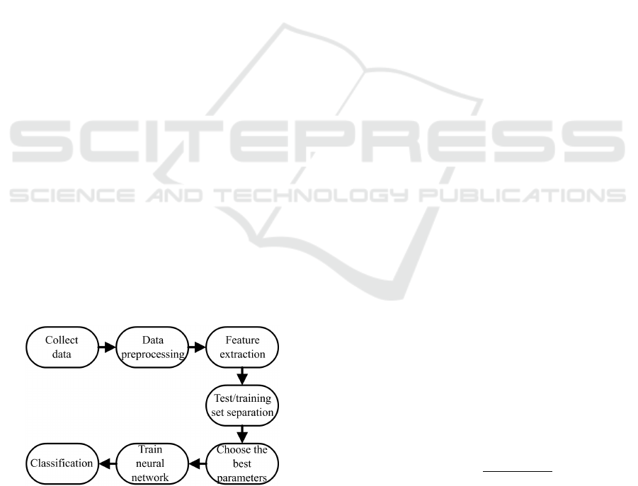
Extraction of relevant features of ECN signals is the
first step for automatic classification of the types of
corrosion that affect the surface of a metal. One of the
tools that can be used in the classification is Artificial
Neural Networks (ANN) and the basic steps of this
approach can be seen in Figure 1.
Figure 1: Basic flowchart of classification using ANN.
The work developed in (Jian et al., 2013) is one of
the few studies known by the authors that used ma-
chine learning techniques to identify types of corro-
sion through ECN. In that study, features extracted
from ECN signals were used to train an ANN type
MLP (Muti-Layer Perceptron) and SVM (Support
Vector Machine) to perform automatic classification
of types of corrosion that occur on the surface of stain-
less steel: pitting and general corrosion, as well as
the identification of passivation (Jian et al., 2013). In
this work, five classifiers will be evaluated, including
MLP and SVM, to identify three types of localized
corrosion (pitting, crevice corrosion and watermark),
as well as the occurrence of passivation on carbon
steel AISI / SAE 1040. The evaluated classifiers are
presented in the following subsections.
3.1 MLP
MLP is an artificial neural network composed by a
set of processing units (artificial neurons) forming
an input layer, one or more intermediate layers (hid-
den) and an output layer. Their training is supervised
and an algorithm of back propagation of error is used
to adjust their weights in order to minimize the dis-
tance between the network response and the desired
response (Haykin, 1998).
3.2 Probabilistic Neural Network
Probabilistic Neural Network (PNN) is a type of neu-
ral network whose transfer functions are gaussian
functions centered on training samples, which allows
the association between the network structure and
probability density functions. In other words, PNN
provides as output the probability of the input pat-
tern to belong to each class. PNN uses the concept
of Parzen estimators and with enough data converges
on the Bayesian Classifier (Masters, 1995).
3.3 kNN
k nearest neighbor (kNN) is a technique of classifica-
tion based on distance (Duda et al., 2000). The learn-
ing in this classifier is based on analogy. To determine
the class of an input pattern, kNN searches the k sam-
ples of the training set that are nearest to the input,
that is, those with the smallest distances. There are
several distance metrics, and the Euclidean distance
is the most common. Equation 13 shows this metric,
where x and y are two samples with n features.
d(x, y) =
s
n
∑
i=1
(x
i
−y
i
)
2
. (13)
3.4 Decision Tree
Decision trees are algorithms used in the classification
of patterns based on the idea of “divide and conquer”:
Identification of Types of Corrosion through Electrochemical Noise using Machine Learning Techniques
335

a complex problem is decomposed into simpler sub-
problems and the same strategy is applied recursively
to each subsub-problem. Thus, the ability of descrip-
tion of a tree comes from dividing the space defined
by the feature in subspaces, where each subspace is
associated with a class. The starting point of a deci-
sion tree is called the root node and consists of all the
learning set, and it is at the top of the tree. A node is
a subset of the features set, and can be terminal (leaf
node) or non-terminal (division node). In the train-
ing process of the tree, the division criterion must be
maximized until a subset is associated with a class
(Quinlan, 1988).
3.5 SVM
Support Vector Machines (SVM) is a machine learn-
ing technique based on mathematical optimization
and statistical learning theory. SVM is also based on
the idea of separation of data through hyperplanes to
determine the class of each sample. To ensure the in-
herent convexity of the optimization problem in the
process of SVM learning, it is necessary to choose
the kernel function that best fits the problem. In this
work is used linear kernel because of its simplicity.
To design the SVM is necessary to determine three
parameters: the cost (c), the kernel function, and ker-
nel parameters, but in the linear kernel does not exist
parameter. The cost is a constant of tolerance to error,
that is, the higher the cost value, the less the error can
be tolerated by learning (Theodoridis and Koutroum-
bas, 2008).
4 MATERIALS AND METHOD TO
COLLECT THE DATA
Corrosion analysis, through signal processing, con-
sists in the mounting of an experimental appara-
tus, called electrochemical cell, and an A/D (ana-
log/digital) converter is used for the measurements
of electrochemical noise. In this work, potential sig-
nals were measured and stored and, indirectly, cur-
rent signals. Electrochemical cell is an experimen-
tal apparatus consisting of an inert metal immersed in
an aqueous solution containing ions in different ox-
idation states. The cell used in this study consists
of two steel electrodes AISI 1040 used as working
electrodes and counter electrodes. These electrodes
are nominally identical and coated with termocon-
tract, and they have exposed area to solution equal to
499,512mm
2
. The reference electrode used to collect
data was Ag/AgCl. Through the A/D converter inter-
face is connected to the electrochemical cell, with the
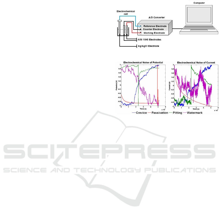
Figure 2: Experimental apparatus configuration.
Figure 3: Collected Electrochemical Signals in Same Scale.
computer, you can store and perform math operations
on the data. Figure 2 shows a diagram with the instru-
ments used for data collection and Figure 3 shows the
ECN signals collected.
According to the American Institute of Iron and
Steel and International Society of Automotive En-
gineers, 1040 steel consists of about 0.37 to 0.44%
carbon (C) 0.6 to 0.9% manganese (Mn) of at
most 0.040% phosphorus (P) and 0.050% sulfur (S).
Among the metals used in the industry, carbon steel
1040 has a wide range of use. Its main applica-
tions are in mechanical components such as gears,
shafts, crankshafts, camshafts, guide pins, gear rings,
columns, turnstiles, cases, construction of oil and gas
pipelines. These structures are subject to corrosion,
and tragic consequences may occur for people who
work in the vicinity of such equipment (Gentil, 2003).
To collect the data, steel electrodes were immersed for
24 hours in passivation solution Na
3
PO
4
with con-
centration of 0.02 M (mol/L), and sampling frequency
of 1 Hz. After that time, the NaCl solution was added
with a concentration of 0.34 M to start the experiment
in aggressive solution for a period of approximately
120 hours and sampling frequency of 1 Hz. All mea-
surements were obtained at room temperature. The
formation and growth of passive film and the occur-
rence of corrosion were analyzed using the potential
and current of the noise according to immersion time.
The electrochemical noise signals of the current and
potential were recorded by an A/D converter.
ICPRAM 2017 - 6th International Conference on Pattern Recognition Applications and Methods
336

5 RESULTS AND DISCUSSION
The experiments were divided into two phases. In the
first phase, the most relevant features were selected
to identify the types of corrosion. This step is impor-
tant to reduce the computational cost and improve the
performance of classifiers. In the second phase, the
classification algorithms are trained with the features
found to identify the occurrence and type of corro-
sion. In both phases, the accuracy metric was used as
quality measure. The value of the accuracy is calcu-
lated by the ratio of the number of samples correctly
classified by the total number of samples, multiplied
by 100%. The higher the value of accuracy, the better.
The best value is 100%.
5.1 Feature Selection
In this phase, the following features (and respective
dimensions) were evaluated: detail and smooth co-
efficients (10 elements each), energy (8 elements),
entropy (9 elements), ratio between standard devia-
tion and mean (1 element), kurtosis (1 element), ra-
tio between the derivative and the mean (1 element),
and resistance to electrochemical noise (1 element).
Each characteristic was extracted for both voltage and
current signals, except resistance to electrochemical
noise. Thus, the full feature vector to be analyzed
by the SBS has 81 elements. The Wavelet Transform
of Daubechies (db4) with decomposition at 8 levels
was used to compute the energy and entropy, as de-
scribed in Section 2.1, in addition to detail and smooth
coefficients. The main property of the Daubechies
function is that it is a wavelet highly localized in
time, which is good for electrochemical noise stud-
ies, where short time duration events are the norm
(Bertocci et al., 1997). The features were obtained
from non-overlapping data packets composed of 1024
points of ECN signals of potential and current.
For the selection of the most significant features,
we used SBS algorithm (Sequential Backward Fea-
ture Selection), which is a search algorithm that starts
with a complete set of features and for each iteration
removes the feature with the least impact on the estab-
lished criterion function (in this paper we used accu-
racy). Multidimensional features has been analyzed
as a group, not individually.
SBS was applied along with a MLP with 20 neu-
rons in the hidden layer, learning rate equal to 0.001
and 1000 training epochs using Levenberg-Marquardt
algorithm (Marquardt, 1963) for training. For this ex-
periment, a training set of 132 samples and a test set
with 68 samples were used, totaling 200 examples se-
lected of different parts of the sampled signal, while
ensuring there is the same number of samples for all
four classes. The features were normalized by the
mean and standard deviation obtained from the train-
ing set, so that the distribution of each feature has zero
mean and standard deviation equal to one.
The attributes selected by the SBS were: entropy,
energy, and resistance to electrochemical noise, re-
sulting in a feature vector of 35 elements (8 entropy
and 9 energy for each voltage and current signal, and
one resistance of the electrochemical noise).
In Figure 4 is shown in 2D graphics how good the
selected features are to separate the samples of the
different types of corrosion. Figure 4(a) shows the
separation using all features and 4(b) using only the
selected features. As we can see, the separation using
the selected features is clearer than using all features.
A dimensionality reduction technique is necessary to
visualize this graphics, whose mapping hold neigh-
borhood relations in the dataset, i.e., if a p instance
is neighbor of q in the original space, the mapped
point p must also be neighbor of q in reduced dimen-
sional space. For this porpose, we used t-Distributed
Stochastic Neighbor Embedding Technique (t-SNE),
which produces one of the best mappings in terms
of preserving neighborhoods (Fadel et al., 2015). t-
SNE is a dimensionality reduction technique based on
probabilities that aims to position multidimensional
data in two-dimensional space, preserving local struc-
tures. In this technique, similarities between pairs
of instances in the original space are modeled as a
distribution of t-student probabilities. More specifi-
cally, the more similar two elements are, the higher
the probability associated with them. Similarly, the
distances between pairs of projected points are also
modeled as a probability distribution.
Two points must be highlighted here. First, al-
though the ratio between the number of samples and
the number of features is low, we can see in Figure
4(b) that the separations among the classes are almost
linear, so complex surfaces are not required for class
separation, and even simple models, such as decision
trees, can perform the task properly with few samples.
Second, although the selected features may favor the
MLP algorithm more than the other ones, previous
experiments have indicated that some of the evalu-
ated features, such as those based on statistics, are
not very useful for this task, and probably other al-
gorithms could have selected the same set of features.
5.2 Corrosion Type Determination
To verify if the selected features have a good ability
to distinguish the different types of corrosion, the next
step is the training of the classifiers presented in Sec-
Identification of Types of Corrosion through Electrochemical Noise using Machine Learning Techniques
337

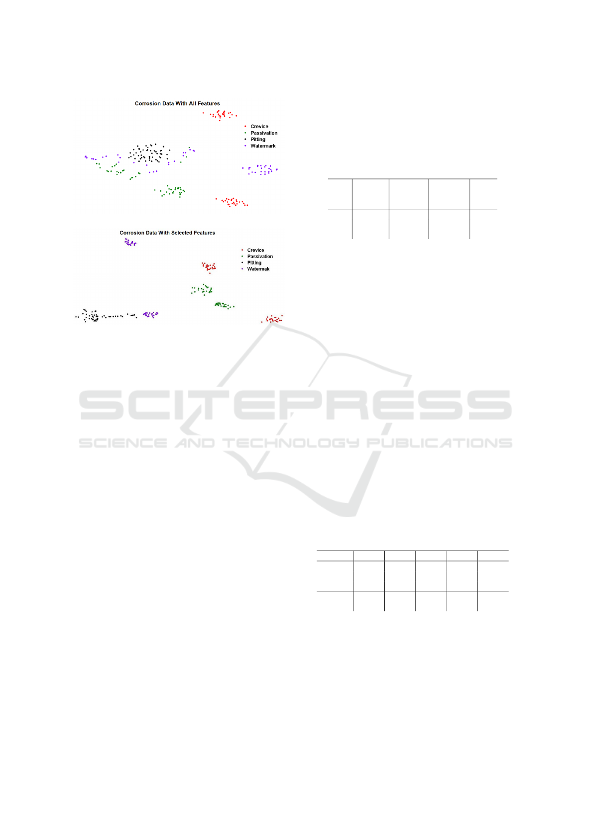
(a)
(b)
Figure 4: Features visualization using t-SNE. Visualizing
corrosion data with (a) all features and (b) selected features.
tion 3. Initially, 48 samples for each one of the four
types of corrosion were obtained, each one composed
of the 35 features selected in Section 5.1. The features
were extracted from non-overlapping data packets of
1024 points each, from potential and current signals.
These packages were selected from different parts of
the sampled signal (which were different to those used
in Section 5.1). After this step, the samples were strat-
ified into 3 folds of data, each one with 64 samples.
Then, for each classifier were obtained 3 results from
3 tests, and each result was achieved using 2 folds for
training/validation and 1 fold for testing. For each re-
sult was used a different fold for testing. The features
were normalized by the mean and standard deviation,
as described in Section 5.1.
The following configurations were tested for each
technique in order to maximize the accuracy on the
training set and, possibly, also on the test set. MLP
was trained using Levenberg-Marquardt algorithm,
learning rate of 0.001, 1000 epochs and evaluated dif-
ferent numbers of neurons in the hidden layer (1 to 50
neurons). Different values of standard deviation were
tested for PNN (0.1 to 1.0, with steps of 0.1). For
kNN, we employed Euclidean distance and we varied
the value of k (1 to 10). The SVM used in the exper-
iments had linear kernel, and different values of cost
c were evaluated (0 to 10, with steps of 0.5). For the
decision tree was used the standard Matlab implemen-
tation, which does not have parameters to tune. For
each test, the parameters of each technique were ad-
justed in order to maximize the accuracy on the train-
ing folds, and these parameters were used to classify
the samples of the test fold. Table 1 shows the values
of the parameters selected for each test fold and for
each classifier.
Table 1: Selected parameter for each classifier.
Test
MLP
Neurons
PNN
Standard
deviation
kNN
k
neighbors
SVM
Cost
1 28 0.3 1 2
2 37 0.2 4 0.5
3 5 0.2 1 0.5
Table 2 shows the values of the accuracy obtained
by each technique in each test fold, and the best re-
sult for each fold was highlighted. The features were
normalized by the mean and standard deviation ob-
tained from the training set. As can be seen, all al-
gorithms have achieved an average accuracy above
95%, with the exception of the decision tree. SVM
achieved mean accuracy slightly better than those ob-
tained by the other classifiers, followed by MLP. kNN
and PNN, which are simpler techniques to implement,
achieved results as good as SVM. Therefore, they are
an option for cases where simplicity is more valuable
than performance. Decision tree achieved high accu-
racy value for the first and third test folds, but for the
second test fold it did not achieve the same perfor-
mance. Some reasons may have been the construc-
tion of a tree with little capability of generalization
and the fact that the process of feature normalization,
through mean and standard deviation, have no effect
on the decision trees. However, the high accuracy val-
ues in other classifiers indicate that this methodology
was effective to identify the types of corrosion ana-
lyzed.
Table 2: Classification results of each technique with nor-
malization (accuracy values are in percent).
Test MLP PNN kNN Tree SVM
1 95.59 97.66 95.31 100.00 100.00
2 100.00 100.00 100.00 78.13 100.00
3 95.31 92.97 92.19 96.88 92.26
Mean 96.97 96.88 95.83 91.67 97.42
Std. Dev. 0.02 0.03 0.03 0.11 0.04
In Table 3 is shown the results of the same ex-
periment, but the features were not normalized. As
we can see, the average accuracy of each classify is
slightly lower than the results shown in Table 2. Thus,
normalized features help to improve the results. How-
ever, all techniques in Table 3 achieved an average ac-
curacy above 90%. Furthermore, as can be observed,
the accuracy of the decision trees are the same in both
tables, because normalization has not effect on them.
ICPRAM 2017 - 6th International Conference on Pattern Recognition Applications and Methods
338

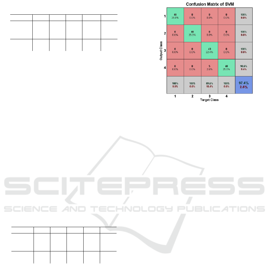
Table 3: Classification results of each technique without
normalization (accuracy values are in percent).
Test MLP PNN kNN Tree SVM
1 92.28 99.22 95.31 100.00 96.87
2 95.44 88.28 93.75 78.13 93.75
3 94.41 94.66 92.69 96.88 95.31
Mean 95.04 94.05 93.92 91.67 95.31
Std. Dev. 0.03 0.06 0.01 0.11 0.01
The results using the selected features were com-
pared to the results obtained with the features used in
(Jian et al., 2013), which is one the few studies known
by the authors that uses features extracted from ECN
signals to train a machine learning technique. The
features used in (Jian et al., 2013) were the elec-
trochemical noise resistance (R
n
), the frequency of
events ( f
n
), the charge (q) and the energy of the de-
tail coefficients extracted by wavelet transform. Us-
ing these features were obtained the results in Table
4, when employing the same previous procedure to
train/validate and test the classifiers (using the same
dataset). The comparison between Tables 2 and 4 in-
dicates that the features used in this work are more
effective to identify correctly the types of corrosion.
The main difference between the two approaches is
the use of entropy information. In (Jian et al., 2013)
is used the Stern-Geary constant, but it can be a great
source of error if this value is not precisely estimated
(Ahmad et al., 2014). Moreover, this value is not con-
stant in some cases (Poursaee, 2010).
Table 4: Classification results of each technique using the
features employed in (Jian et al., 2013) (accuracy values are
in percent).
Test MLP PNN kNN Tree SVM
1 89.06 84.38 73.44 70.31 71.87
2 85.15 89.84 82.81 76.56 85.93
3 76.56 78.13 70.31 64.06 53.12
Mean 83.59 84.11 75.52 70.31 70.31
Std. Dev. 0.06 0.05 0.06 0.06 0.16
For a better analyze of the results, the average ac-
curacy of the SVM in Table 2 is shown in a confusion
matrix (Figure 5). Each column in this matrix is a out-
put class and each row is a target class. In the diago-
nal of matrix (in green) are shown the outputs that are
equal to the target classes. The red elements indicate
the wrong outputs. The gray boxes are the accuracy
of each corrosion type, and the blue box is the average
accuracy of the SVM. The numbers 1, 2, 3 and 4 in-
dicate the crevice, passivation, pitting and watermark
classes, respectively. Observing the confusion matrix
is possible to identify that only 5 samples belonging
to pitting class were wrong classified as watermark by
the SVM. This error could be expected by inspecting
Figure 4(b), where we can see a little separation mar-
gin between pitting and watermark.
Figure 5: Confusion matrix of SVM.
6 CONCLUSIONS
This paper presented an approach to identify some
types of corrosion on metal surface through electro-
chemical noise signals. In experimental results was
observed that resistance to electrochemical noise and
features extracted from wavelet transform, entropy
and energy, were the most discriminative for this task.
After analyzing the results for the five evaluated clas-
sifiers, we noted that all five algorithms had achieved
an average accuracy above 90% to perform the task,
and SVM achieved an average accuracy slightly better
than those obtained by the other classifiers for iden-
tifying types of corrosion. Therefore, the results of
this study highlight the importance of using wavelet
transform for electrochemical noise analysis. In fu-
ture work, we intend to analyze other algorithms and
other features in order to improve the results using
only a type of signal, simplifying the instrumentation
necessary to collect the data.
ACKNOWLEDGEMENTS
Lorraine Marques Alves would like to thank CAPES
for the scholarship granted.
REFERENCES
Aballe, A., Bethencourt, M., Botana, F., and Marcos, M.
(1999). Using wavelets transform in the analysis of
electrochemical noise data. In Electrochimica Acta.
Elsevier.
Ahmad, S., Jibran, M. A. A., Azad, A. K., and Maslehud-
din, M. (2014). A simple and reliable setup for mon-
Identification of Types of Corrosion through Electrochemical Noise using Machine Learning Techniques
339

itoring corrosion rate of steel rebars in concrete. The
Scientific World Journal, page 10.
Amaya, J., Cottis, R. A., and Botana, F. (2005). Shot noise
and statistical parameters for the estimation of corro-
sion mechanisms. In Corrosion Science. Elsevier.
Barr, E., Greenfield, A., and Pierrard, L. (2001). Applica-
tion of electrochemical noise monitoring to inhibitor
evaluation and optimization in the field: Results from
the kaybob south sour gas field. In Corrosion. NACE
international.
Bertocci, U., Gabrielli, C., Huet, F., and Keddan, M. (1997).
Noise resistance applied to corrosion measurements.
In Electrochemical Society Journal. electrochemical
Society.
Cottis, R. (2001). Interpretation of electrochemical noise
data. In Corrosion. NACE international.
Cottis, R. and Turgoose, S. (1999). Corrosion Testing Made
Easy: Impedance and Noise Analysis. NACE Interna-
tional, Houston, 1nd edition.
Cottis, R. A., Homborg, A., and Mol, J. (2015). The rela-
tionship between spectral and wavelet techniques for
noise analysis. In Electrochimica Acta. Elsevier.
Cox, W. M. (2014). A strategic approach to corrosion mon-
itoring and corrosion management. Procedia Engi-
neering, 86:567–575.
Duda, R., Hart, D. G., and Stork, P. (2000). Pattern Recog-
nition. Wiley Interscience, New York, 1nd edition.
Fadel, S. G., Fatore, M., Duarte, S., and Paulovich,
V. (2015). Loch: A neighborhood-based multidi-
mensional projection technique for high-dimensional
sparse spaces. In Neurocomputing. Elsevier.
Fernandes, J., Kubota, L., and Neto, G. (2001). Ion-
selective eletrodes: historical, mechanism of re-
sponse, selectivity and concept review. In Quimica
Nova. Scielo.
Fofano, S. and Jambo, H. (2007). Corrosion: fundamentals,
monitoration and control. Ciencia Moderna, Brazil,
1nd edition.
Gentil, V. (2003). Corrosion. LTC, Brazil, 1nd edition.
Haykin, S. (1998). Neural Networks: A Comprehensive
Foundation. Prentice Hall, Canada, 2nd edition.
Jian, L., Weikang, K., Jiangbo, S., Ke, W., Weikui, W.,
Z.Weipu, and Zhoumo, Z. (2013). Determination of
corrosion types from electrochemical noise by artifi-
cial neural networks. In international Journal of Elec-
trochemical Science. Electrochemical Science.
Kim, J. (2007). Wavelet analysis of potentiostatic electro-
chemical noise. In Materials Letters. Elsevier.
Koch, G., Varney, J., Thompson, N., Moghissi, O., Gould,
M., and Payer, J. (2016). International measures
of prevention, application and economics of corro-
sion technologies study (impact). In Technical report.
NACE international.
Marquardt, D. W. (1963). An algorithm for least-squares
estimation of nonlinear parameters. Journal of
the Society for Industrial and Applied Mathematics,
11(2):431–441.
Masters, T. (1995). Advanced algorithms for Neural Net-
works: A C++ Sourcebook. John Wiley and Sonsl,
New York, 1nd edition.
Moshrefi, R., Mahjani, M., and Jafarian, M. (2014). Appli-
cation of wavelet entropy in analysis of electrochemi-
cal noise for corrosion type identification. In Electro-
chemistry Communications. Elsevier.
Planinsic, P. and Petek, A. (2008). Characterization of cor-
rosion process by current noise-based fractal and cor-
relation analysis. In Electrochimica Acta. Elsevier.
Poursaee, A. (2010). Potentiostatic transient technique,
a simple approach to estimate the corrosion cur-
rent density and stern-geary constant of reinforcing
steel in concrete. Cement and Concrete Research,
40(9):1451–1458.
Quinlan, J. (1988). Decision trees and multivalued at-
tributes. Oxford University Press, New York, 11nd
edition.
Research, E. P. A. (1980). Basics of corrosion measure-
ments - application note corr-1. Technical report,
Princeton.
Rios, E., Zimer, A., Pereira, E., and Mascaro, L. (2013).
Analysis of aisi 1020 steel corrosion in seawater
by coupling electrochemical noise and optical mi-
croscopy. In Electrochimica Acta. Elsevier.
Smulko, J., Darowicki, K., and Zielinski, A. (2002). Pitting
corrosion in steel and electrochemical noise intensity.
In Electrochemistry Communication. Elsevier.
Theodoridis, S. and Koutroumbas, K. (2008). Pattern
Recognition. Elsevier, San Diego, 4nd edition.
Wharton, A., Woo, R. J. K., and Mellor, B. G. (2002).
Wavelet analysis of electrochemical noise measure-
ments during corrosion of austenitic and superduplex
stainless steels in chloride media. In Corrosion Sci-
ence. Elsevier.
ICPRAM 2017 - 6th International Conference on Pattern Recognition Applications and Methods
340