
How New Information Criteria WAIC and WBIC
Worked for MLP Model Selection
Seiya Satoh
1
and Ryohei Nakano
2
1
National Institute of Advanced Industrial Science and Tech, 2-4-7 Aomi, Koto-ku, Tokyo, 135-0064, Japan
2
Chubu University, 1200 Matsumoto-cho, Kasugai, 487-8501, Japan
seiya.satoh@aist.go.jp, nakano@cs.chubu.ac.jp
Keywords:
Information Criteria, Model Selection, Multilayer Perceptron, Singular Model.
Abstract:
The present paper evaluates newly invented information criteria for singular models. Well-known criteria
such as AIC and BIC are valid for regular statistical models, but their validness for singular models is not
guaranteed. Statistical models such as multilayer perceptrons (MLPs), RBFs, HMMs are singular models.
Recently WAIC and WBIC have been proposed as new information criteria for singular models. They are
developed on a strict mathematical basis, and need empirical evaluation. This paper experimentally evaluates
how WAIC and WBIC work for MLP model selection using conventional and new learning methods.
1 INTRODUCTION
A statistical model is called regular if the mapping
from a parameter vector to a probability distribution
is one-to-one and its Fisher information matrix is al-
ways positive definite; otherwise, it is called singular.
Many useful statistical models such as multilayer per-
ceptrons (MLPs), RBFs, HMMs, Gaussian mixtures,
are all singular.
Given data, we sometimes have to select the best
statistical model that has the optimum trade-off be-
tween goodness of fit and model complexity. This
task is called model selection, and many information
criteria have been proposed as measures for this task.
Most information criteria such as AIC (Akaike’s
information criterion) (Akaike, 1974), BIC (Bayesian
information criterion) (Schwarz, 1978), and BPIC
(Bayesian predictive information criterion) (Ando,
2007) are for regular models. These criteria assume
the asymptotic normality of maximum likelihood es-
timator; however, in singular models this assumption
does not hold any more. Recently Watanabe estab-
lished singular learning theory (Watanabe, 2009), and
proposed new criteria WAIC (widely applicable infor-
mation criteria) (Watanabe, 2010) and WBIC (widely
applicable Bayesian information criterion) (Watan-
abe, 2013), applicable to singular models. WAIC and
WBIC have been developed on a strict mathematical
basis, and how they work for singular models needs
to be investigated hereafter.
Let MLP(J) be an MLP having J hidden units;
note that an MLP model is determined by the num-
ber J. When evaluating MLP model selection ex-
perimentally, we have to run learning methods for
different MLP models. There can be two ways to
perform this learning: independent learning and suc-
cessive learning. In the former, we run a learn-
ing method repeatedly and independently for each
MLP(J), whereas in the latter MLP(J) learning in-
herits solutions from MLP(J−1) learning. As J gets
larger, a model gets more complex having more fitting
capability. This means training error should mono-
tonically decrease as J gets larger. However, inde-
pendent learning will not guarantee this monotonic-
ity. A new learning method called SSF (Singularity
Stairs Following) (Satoh and Nakano, 2013a; Satoh
and Nakano, 2013b) realizes successive learning by
utilizing singular regions to stably find excellent so-
lutions, and can guarantee the monotonicity.
This paper experimentally evaluates how new cri-
teria WAIC and WBIC work for MLP model selec-
tion, compared with conventional criteria AIC and
BIC, using a conventional learning method called
BPQ (Back Propagation based on Quasi-Newton)
(Saito and Nakano, 1997) and the new learning
method SSF for search and sampling. BPQ is a
kind of quasi-Newton method with BFGS (Broyden-
Fletcher-Goldfarb-Shanno) update.
Satoh, S. and Nakano, R.
How New Information Criteria WAIC and WBIC Worked for MLP Model Selection.
DOI: 10.5220/0006120301050111
In Proceedings of the 6th International Conference on Pattern Recognition Applications and Methods (ICPRAM 2017), pages 105-111
ISBN: 978-989-758-222-6
Copyright
c
2017 by SCITEPRESS – Science and Technology Publications, Lda. All rights reserved
105

2 INFORMATION CRITERIA
FOR MODEL SELECTION
Let a statistical model be p(x|w), where x is an input
vector and w is a parameter vector. Let given data be
D = {x
µ
, µ = 1, ··· , N}, where N indicates data size,
the number of data points.
AIC and BIC:
AIC (Akaike information criterion) (Akaike, 1974)
and BIC (Bayesian information criterion) (Schwarz,
1978) are famous information criteria for regular
models. Both deal with the trade-off between good-
ness of fit and model complexity.
The log-likelihood is defined as follow:
L
N
(w) =
N
∑
µ=1
log p(x
µ
|w). (1)
Let
b
w be a maximum likelihood estimator. AIC is
given below as an estimator of a compensated log-
likelihood using the asymptotic normality of
b
w. Here
M is the number of parameters.
AIC = −2L
N
(
b
w) + 2M
= −2
N
∑
µ=1
log p(x
µ
|
b
w) + 2M (2)
BIC is obtained as an estimator of free energy
F(D) shown below. Here p(D) is called evidence and
p(w) is a prior distribution of w.
F(D) = −log p(D), (3)
p(D) =
Z
p(w)
N
∏
µ=1
p(x
µ
|w) dw (4)
BIC is derived using the asymptotic normality and
Laplace approximation.
BIC = −2L
N
(
b
w) + M logN
= −2
N
∑
µ=1
log p(x
µ
|
b
w) + M logN (5)
AIC and BIC can be calculated using only one point
estimator
b
w.
WAIC and WBIC:
WAIC and WBIC are derived from Watanabe’s sin-
gular learning theory (Watanabe, 2009) as new infor-
mation criteria for singular models. Watanabe intro-
duced the following four quantities: Bayes general-
ization loss BL
g
, Bayes training loss BL
t
, Gibbs gen-
eralization loss GL
g
, and Gibbs training loss GL
t
.
BL
g
= −
Z
p
∗
(x) log p(x|D)dx (6)
BL
t
= −
1
N
N
∑
µ=1
log p(x
µ
|D) (7)
GL
g
= −
Z
Z
p
∗
(x)log p(x|w)dx
p(w|D)dw (8)
GL
t
= −
Z
1
N
N
∑
µ=1
log p(x
µ
|w)
!
p(w|D)dw (9)
Here p
∗
(x) is the true distribution, p(w|D) is a poste-
rior distribution, and p(x|D) is a predictive distribu-
tion.
p(w|D) =
1
p(D)
p(w)
N
∏
µ=1
p(x
µ
|w) (10)
p(x|D) =
Z
p(x|w) p(w|D) dw (11)
WAIC1 and WAIC2 are given as estimators of BL
g
and GL
g
respectively (Watanabe, 2010). WAIC1 re-
duces to AIC for regular models.
WAIC1 = BL
t
+ 2(GL
t
− BL
t
) (12)
WAIC2 = GL
t
+ 2(GL
t
− BL
t
) (13)
WBIC is given as an estimator of free energy F(D) for
singular models (Watanabe, 2013), where p
β
(w|D) is
a posterior distribution under the inverse temperature
β. In WBIC context, β is set to be 1/log(N). WBIC
reduces to BIC for regular models.
WBIC = −
Z
N
∑
µ=1
log p(x
µ
|w)
!
p
β
(w|D)dw (14)
p
β
(w|D) =
1
p
β
(D)
p(w)
N
∏
µ=1
p(x
µ
|w)
β
(15)
There are two ways to calculate WAIC and WBIC:
analytic approach and empirical one. We employ the
latter, which requires a set of weights {w
t
} which ap-
proximates a posterior distribution (Watanabe, 2009).
3 SSF: NEW LEARNING
METHOD
SSF (Singularity Stairs Following) is briefly ex-
plained; for details, refer to (Satoh and Nakano,
2013a; Satoh and Nakano, 2013b). SSF finds so-
lutions of MLP(J) successively from J=1 until J
max
making good use of singular regions of each MLP(J).
Singular regions of MLP(J) are created by utilizing
the optimum of MLP(J−1). Gradient is zero all over
the region.
How to create singular regions is explained be-
low. Consider MLP(J) with just one output unit
which outputs f
J
(x;θ
J
) = w
0
+
∑
J
j=1
w
j
z
j
, where θ
J
ICPRAM 2017 - 6th International Conference on Pattern Recognition Applications and Methods
106

= {w
0
,w
j
,w
j
, j = 1, ··· , J}, z
j
≡ g(w
T
j
x), and g(h)
is an activation function. Given data {(x
µ
,y
µ
),µ =
1,· · · ,N}, we try to find MLP(J) which minimizes
an error function. We also consider MLP(J−1)
with θ
J−1
= {u
0
,u
j
,u
j
, j = 2,··· , J}. The output is
f
J−1
(x;θ
J−1
) = u
0
+
∑
J
j=2
u
j
v
j
, where v
j
≡ g(u
T
j
x)
Now consider the following reducibility mappings
α, β, and γ. Then apply α, β, and γ to the optimum
b
θ
J−1
to get regions
b
ϑ
α
J
,
b
ϑ
β
J
, and
b
ϑ
γ
J
respectively.
b
θ
J−1
α
−→
b
ϑ
α
J
,
b
θ
J−1
β
−→
b
ϑ
β
J
,
b
θ
J−1
γ
−→
b
ϑ
γ
J
b
ϑ
α
J
≡{θ
J
|w
0
=
b
u
0
, w
1
=0,
w
j
=
b
u
j
,w
j
=
b
u
j
, j =2, ··· , J}
b
ϑ
β
J
≡{θ
J
|w
0
+w
1
g(w
10
)=
b
u
0
,
w
1
=[w
10
,0, ...,0]
T
,
w
j
=
b
u
j
,w
j
=
b
u
j
, j = 2, ...,J}
b
ϑ
γ
J
≡{θ
J
|w
0
=
b
u
0
,w
1
+w
m
=
b
u
m
,
w
1
=w
m
=
b
u
m
,
w
j
=
b
u
j
,w
j
=
b
u
j
, j ∈ {2, ...,J}\m}
Now two singular regions can be formed. One is
b
ϑ
αβ
J
,
the intersection of
b
ϑ
α
J
and
b
ϑ
β
J
. The parameters are
as follows, where only w
10
is free: w
0
=
b
u
0
, w
1
=
0, w
1
= [w
10
,0, ··· ,0]
T
,w
j
=
b
u
j
, w
j
=
b
u
j
, j =
2,· · · ,J. The other is
b
ϑ
γ
J
, which has the restriction:
w
1
+ w
m
=
b
u
m
.
SSF starts search from MLP(J=1) and then gradu-
ally increases J one by one until J
max
. When start-
ing from the singular region, the method employs
eigenvector descent (Satoh and Nakano, 2012), which
finds descending directions, and from then on em-
ploys BPQ (Saito and Nakano, 1997), a quasi-Newton
method. SSF finds excellent solution of MLP(J) one
after another for J=1,···,J
max
. Thus, SSF guarantees
that training error decreases monotonically as J gets
larger, which will be quite preferable for model selec-
tion.
4 EXPERIMENTS
Experimental Conditions:
We used artificial data since they are easy to control
and their true nature is obvious. The structure of an
MLP is defined as follows: the numbers of input, hid-
den, and output units are K, J, and I respectively.
Both input and hidden layers have a bias. Values
of input data were randomly selected from the range
[0, 1]. Artificial data 1 and data 2 were generated
using MLP(K = 5, J = 20, I = 1) and MLP(K = 10,
J = 20, I = 1) respectively. Weights between input
and hidden layers were set to be integers randomly
selected from the range [−10, +10], whereas weights
between hidden and output layers were integers ran-
domly selected from [−20, +20]. A small Gaussian
noise with mean zero and standard deviation 0.02 was
added to each MLP output. Size of training data was
set to be N = 800, whereas test data size was set to be
1,000.
WAIC and WBIC were compared with AIC
and BIC. The empirical approach needs a sam-
pling method; however, usual MCMC (Markov chain
Monte Carlo) methods such as Metropolis algorithm
will not work at all (Neal, 1996) since MLP search
space is quite hard to search. Thus, we employ power-
ful learning methods BPQ and SSF as sampling meth-
ods. For AIC and BIC a learning method runs with-
out any regularizer, whereas WAIC and WBIC need a
weight decay regularizer whose regularization coeffi-
cient λ depends on temperature T . The temperature T
was set as suggested in (Watanabe, 2010; Watanabe,
2013): T = 1 for WAIC and T = log(N) for WBIC.
The regularization coefficient λ of WAIC is smaller
than that of WBIC. WAIC and WBIC were calculated
using a set of weights {w
t
} approximating a posterior
distribution. Test error was calculated using test data.
Our various previous experiments have shown that
BPQ (Saito and Nakano, 1997) finds much better so-
lutions than BP (Back Propagation) does, mainly be-
cause BPQ is a quasi-Newton, a 2nd-order method.
Thus, we employ BPQ as a conventional learning
method. We performed BPQ independently 100 times
changing initial weights for each J. Moreover, we em-
ploy a newly invented learning method called SSF as
well. For SSF, the maximum number of search routes
was set to be 100 for each J; J was changed from 1
until 24. Each run of a learning method was termi-
nated when the number of sweeps exceeded 10,000
or the step length got smaller than 10
−16
.
Experimental Results:
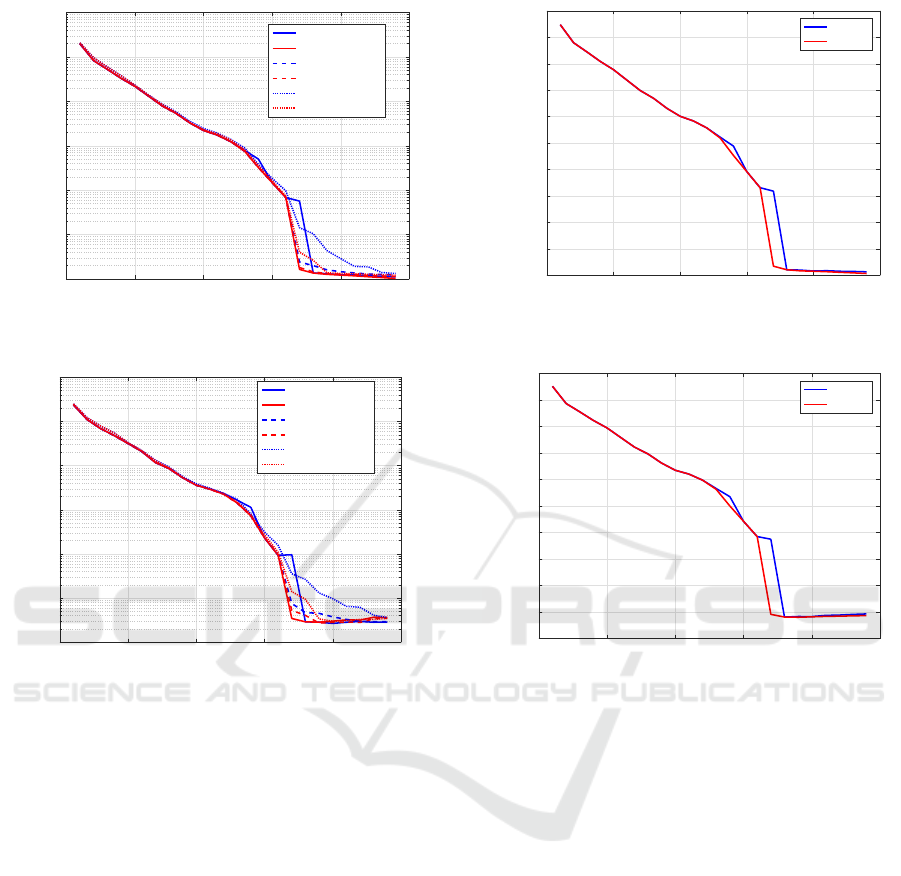
Figures 1 to 6 show a set of results for artificial data
1. Figure 1 shows minimum training error obtained
by each learning method for each J. Although SSF
guarantees the monotonic decrease of minimum train-
ing error, BPQ does not in general. However, BPQ
showed the monotonic decrease for this data. Figure
2 shows test error for
b
w of the best model obtained
by each learning method for each J. BPQ with λ =
0, BPQ with λ for WAIC, and BPQ with λ for WBIC
got the minimum test error at J = 20, 24, and 24 re-
spectively. SSF with λ = 0, SSF with λ for WAIC, and
SSF with λ for WBIC found the minimum test error
at J = 18, 19, and 20 respectively.
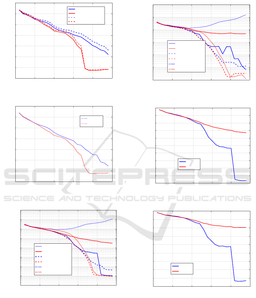
Figure 3 shows AIC values obtained by each
How New Information Criteria WAIC and WBIC Worked for MLP Model Selection
107
0 5 10 15 20 25
Number of Hidden Units
10
-1
10
0
10
1
10
2
10
3
10
4
10
5
Training Error
BPQ (λ =0)
SSF1.4 (λ =0)
BPQ (WAIC)
SSF1.4 (WAIC)
BPQ (WBIC)
SSF1.4 (WBIC)
Figure 1: Training Error for Data 1.
0 5 10 15 20 25
Number of Hidden Units
10
0
10
1
10
2
10
3
10
4
10
5
10
6
Test Error
BPQ (λ =0)
SSF1.4 (λ =0)
BPQ (WAIC)
SSF1.4 (WAIC)
BPQ (WBIC)
SSF1.4 (WBIC)
Figure 2: Test Error for Data 1.
learning method for each J. AIC of both methods se-
lected J ≥ 24 as the best model, which is not suitable
at all. Figure 4 shows BIC values obtained by each
learning method for each J. BIC of BPQ selected J
= 18 as the best model, whereas BIC of SSF selected
J = 19. Thus, BIC selected a bit smaller models than
the true one for this data.
Figure 5 shows WAIC1 and WAIC2 values ob-
tained by each learning method for each J. WAIC1
and WAIC2 of BPQ selected J ≥ 24 as the best model,
which is not suitable. WAIC1 and WAIC2 of SSF se-
lected J = 19 as the best model, which is very close to
the true one (J = 20). WAIC1 and WAIC2 selected the
same model for each method. Figure 6 shows WBIC
values obtained by each learning method for each J.
WBIC of BPQ selected J ≥ 24, which is not suitable,
whereas WBIC of SSF selected J = 20, which is right.
Figures 7 to 12 show the results for artificial data
2. Figure 7 shows minimum training error. SSF
showed the monotonic decrease, whereas BPQ did not
for WBIC. Figure 8 shows test error for
b
w of the best
model obtained by each learning method. BPQ with
0 5 10 15 20 25
Number of Hidden Units
-1000
0
1000
2000
3000
4000
5000
6000
7000
8000
9000
Criterion AIC
BPQ
SSF1.4
Figure 3: AIC for Data 1.
0 5 10 15 20 25
Number of Hidden Units
-500
0
500
1000
1500
2000
2500
3000
3500
4000
4500
Criterion BIC
BPQ
SSF1.4
Figure 4: BIC for Data 1.
λ = 0, λ for WAIC, and λ for WBIC got the minimum
test error at J = 24, 23, and 9 respectively. SSF with λ
= 0, λ for WAIC, and λ for WBIC found the minimum
test error at J = 23, 20, and 24 respectively.
Figure 9 shows AIC values obtained by each
learning method for each J. AIC of BPQ and SSF
selected J = 23 and J ≥ 24 respectively as the best
model, which is not acceptable. Figure 10 shows BIC
values obtained by each learning method for each J.
BIC of BPQ and SSF selected J = 22 and J = 21 re-
spectively as the best model. BIC selected a bit larger
models for this data.
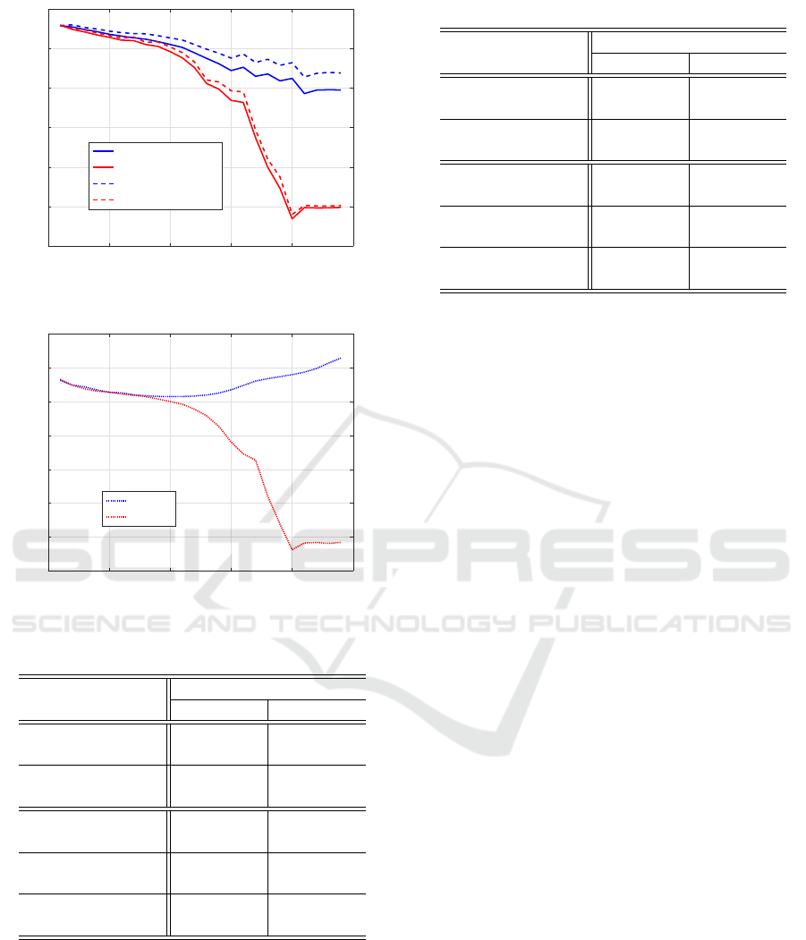
Figure 11 shows WAIC1 and WAIC2 values ob-
tained by each learning method for each J. WAIC1
and WAIC2 of BPQ selected J = 21 as the best model,
which is very close to the true model. WAIC1 and
WAIC2 of SSF selected J = 20 as the best model,
which is exactly the true one. For this data WAIC1
and WAIC2 again selected the same model for each
method. Figure 12 shows WBIC values obtained by
each learning method for each J. WBIC of BPQ se-
lected J = 10, which is quite unacceptable, whereas
ICPRAM 2017 - 6th International Conference on Pattern Recognition Applications and Methods
108
0 5 10 15 20 25
Number of Hidden Units
-3
-2
-1
0
1
2
3
4
Criterion WAIC
BPQ (WAIC 1)
SSF 1.4 (WAIC 1)
BPQ (WAIC 2)
SSF 1.4 (WAIC 2)
Figure 5: WAIC for Data 1.
0 5 10 15 20 25
Number of Hidden Units
-3
-2
-1
0
1
2
3
4
Criterion WBIC
×10
4
BPQ
SSF 1.4
Figure 6: WBIC for Data 1.
0 5 10 15 20 25
Number of Hidden Units
10
-2
10
-1
10
0
10
1
10
2
10
3
10
4
10
5
10
6
Training Error
BPQ (λ =0)
SSF1.4 (λ =0)
BPQ (WAIC)
SSF1.4 (WAIC)
BPQ (WBIC)
SSF1.4 (WBIC)
Figure 7: Training Error for Data 2.
WBIC of SSF selected J = 20, which is just the same
as the true one.
Tables 1 and 2 summarize our results of model
selection using BPQ and SSF for artificial data 1 and
2 respectively.
0 5 10 15 20 25
Number of Hidden Units
10
1
10
2
10
3
10
4
10
5
10
6
10
7
Test Error
BPQ (λ =0)
SSF1.4 (λ =0)
BPQ (WAIC)
SSF1.4 (WAIC)
BPQ (WBIC)
SSF1.4 (WBIC)
Figure 8: Test Error for Data 2.
0 5 10 15 20 25
Number of Hidden Units
-1000
0
1000
2000
3000
4000
5000
6000
7000
8000
9000
Criterion AIC
BPQ
SSF1.4
Figure 9: AIC for Data 2.
0 5 10 15 20 25
Number of Hidden Units
0
500
1000
1500
2000
2500
3000
3500
4000
4500
Criterion BIC
BPQ
SSF1.4
Figure 10: BIC for Data 2.
Considerations:
The results of our experiments may suggest the fol-
lowing. Note, however, that since our experiments
are quite limited, more intensive investigation will be
needed to make the tendencies more reliable.
How New Information Criteria WAIC and WBIC Worked for MLP Model Selection
109
0 5 10 15 20 25
Number of Hidden Units
-2
-1
0
1
2
3
4
Criterion WAIC
BPQ (WAIC 1)
SSF 1.4 (WAIC 1)
BPQ (WAIC 2)
SSF 1.4 (WAIC 2)
Figure 11: WAIC for Data 2.
0 5 10 15 20 25
Number of Hidden Units
-2
-1
0
1
2
3
4
5
Criterion WBIC
×10
4
BPQ
SSF 1.4
Figure 12: WBIC for Data 2.
Table 1: Comparison of Selected Models for Data 1.
learning method
criterion BPQ SSF
AIC ≥24 ≥24
BIC 18 19
WAIC1 ≥24 19
WAIC2 ≥24 19
WBIC ≥24 20
(a) Independent learning of BPQ does not guarantee
monotonic decrease of training error along with the
increase of J, whereas successive learning of SSF
does guarantee the monotonic decrease. For MLP
model selection, independent learning sometimes
did not work well, showing an up-and-down curve
of training error and leading to wrong selection,
whereas successive learning seems suited for MLP
Table 2: Comparison of Selected Models for Data 2.
learning method
criterion BPQ SSF
AIC 23 ≥24
BIC 22 21
WAIC1 21 20
WAIC2 21 20
WBIC 10 20
model selection due to the monotonic decrease of
training error.
(b) In our experiments AIC had the tendency to
select the largest (J ≥ 24) among the candidates
for any learning method. This is probably because
the penalty for model complexity is too small. BIC
worked relatively well, having the tendency to select
a bit smaller or larger models than the true one.
(c) WAIC and WBIC of SSF worked very well, se-
lecting the true model or models very close to the true
one. However, WAIC and WBIC of BPQ sometimes
didn’t work well. Moreover, there was little differ-
ence between WAIC1 and WAIC2 for each learning
method in our experiments.
5 CONCLUSION
WAIC and WBIC are new information criteria for sin-
gular models. This paper evaluates how they work for
MLP model selection using artificial data. We com-
pared them with AIC and BIC using sampling meth-
ods. For this sampling, we used independent learning
of a conventional learning method BPQ and succes-
sive learning of a newly invented SSF. Our experi-
ments showed that WAIC and WBIC of SSF worked
very well, selecting the true model or very close mod-
els for each data, although WAIC and WBIC of BPQ
sometimes did not work well. AIC did not work well
selecting larger models, and BIC had the tendency to
select a bit smaller or larger models. In the future we
plan to do more intensive investigation on WAIC and
WBIC.
ICPRAM 2017 - 6th International Conference on Pattern Recognition Applications and Methods
110

ACKNOWLEDGEMENT
This work was supported by Grants-in-Aid for Scien-
tific Research (C) 16K00342.
REFERENCES
Akaike, H. (1974). A new look at the statistical model iden-
tification. IEEE Trans. on Automatic Control, AC-
19:716–723.
Ando, T. (2007). Bayesian predictive information criterion
for the evaluation of hierarchical Bayesian and empir-
ical Bayes models. Biometrika, 94:443–458.
Neal, R. (1996). Bayesian learning for neural networks.
Springer.
Saito, K. and Nakano, R. (1997). Partial BFGS update and
efficient step-length calculation for three-layer neural
networks. Neural Comput., 9(1):239–257.
Satoh, S. and Nakano, R. (2012). Eigen vector descent
and line search for multilayer perceptron. In IAENG
Int. Conf. on Artificial Intelligence & Applications
(ICAIA’12), volume 1, pages 1–6.
Satoh, S. and Nakano, R. (2013a). Fast and stable learn-
ing utilizing singular regions of multilayer perceptron.
Neural Processing Letters, 38(2):99–115.
Satoh, S. and Nakano, R. (2013b). Multilayer perceptron
learning utilizing singular regions and search pruning.
In Proc. Int. Conf. on Machine Learning and Data
Analysis, pages 790–795.
Schwarz, G. (1978). Estimating the dimension of a model.
Annals of Statistics, 6:461–464.
Watanabe, S. (2009). Algebraic geometry and statistical
learning theory. Cambridge University Press, Cam-
bridge.
Watanabe, S. (2010). Equations of states in singular statis-
tical estimation. Neural Networks, 23:20–34.
Watanabe, S. (2013). A widely applicable Bayesian infor-
mation criterion. Journal of Machine Learning Re-
search, 14:867–897.
How New Information Criteria WAIC and WBIC Worked for MLP Model Selection
111
