Recognition of Handwritten Music Symbols using Meta-features

Obtained from Weak Classiﬁers based on Nearest Neighbor

Jorge Calvo-Zaragoza, Jose J. Valero-Mas and Juan R. Rico-Juan

Department of Software and Computing Systems, University of Alicante,

Carretera San Vicente del Raspeig s/n, Alicante, Spain

{jcalvo, jjvalero, juanra}@dlsi.ua.es

Keywords:

Optical Music Recognition, Music Symbols, Handwriting Recognition, Symbol Classiﬁcation, Meta-features

Space.

Abstract:

The classiﬁcation of musical symbols is an important step for Optical Music Recognition systems. However,

little progress has been made so far in the recognition of handwritten notation. This paper considers a scheme

that combines ideas from ensemble classiﬁers and dissimilarity space to improve the classiﬁcation of hand-

written musical symbols. Several sets of features are extracted from the input. Instead of combining them,

each set of features is used to train a weak classiﬁer that gives a conﬁdence for each possible category of the

task based on distance-based probability estimation. These conﬁdences are not combined directly but used

to build a new set of features called Conﬁdence Matrix, which eventually feeds a ﬁnal classiﬁer. Our work

demonstrates that using this set of features as input to the classiﬁers signiﬁcantly improves the classiﬁcation

results of handwritten music symbols with respect to other features directly retrieved from the image.

1 INTRODUCTION

Composing music with pen and paper is still a com-

mon procedure for most musicians. Nevertheless,

digital versions of music scores offer a great deal of

advantages with respect to the physical ones. For

instance, issues related to the storage, distribution,

preservation, and reproduction of the information are

straightforwardly solved in the digital domain. Also,

having such music information encoded in a struc-

tured format opens the possibility of applying com-

putational music tools for tasks such as content-based

music searches, musicological analysis or organiza-

tion in digital libraries, among others.

In order to take advantage of the aforementioned

processes, handwritten scores need to be transcribed

onto a digital version. Most commonly, this is done

by hand using some kind of software for music score

edition. Unfortunately, the process can be very te-

dious since the complexity of music notation in-

evitably leads to burdensome and uncomfortable in-

terfaces based on drag and drop actions with the

mouse.

An effortless alternative for the user to obtain the

digital version of a handwritten music composition is

to resort to an Optical Music Recognition (OMR) sys-

tem (Bainbridge and Bell, 2001). These systems im-

port a scanned version of the music sheet and try to

automatically export the information to some type of

machine-readable format such as MusicXML, MIDI

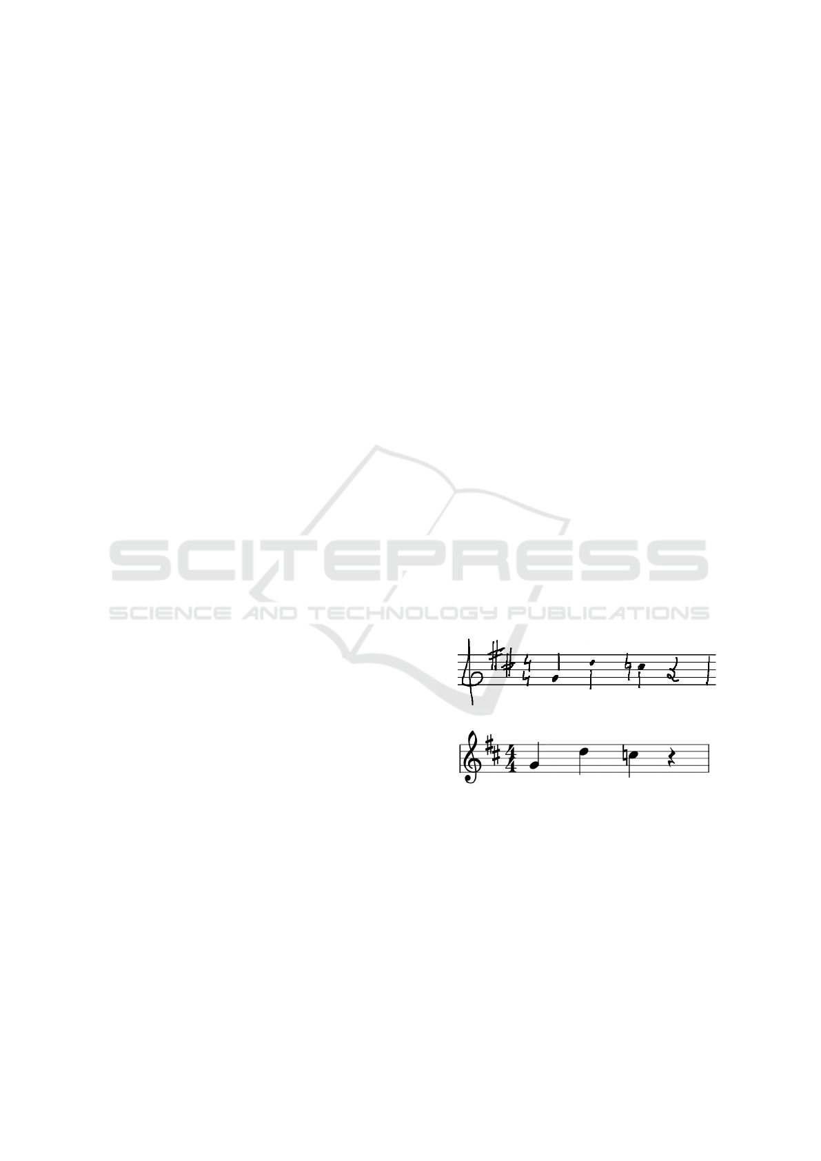
or MEI (see Fig. 1).

(a) Example of input score for an OMR system

(b) Symbolic representation of the input score

Figure 1: The task of Optical Music Recognition (OMR) is

to analyze an image containing a music score to export its

musical content into some machine-readable format.

Given the particularities of music notation, an

OMR system usually follows a segmentation-based

approach: isolated symbols are initially detected and,

then, classiﬁed. The process starts with a preprocess-

ing stage, which focuses on providing robustness to

the system by means of binarization and deskewing.

Then, a process for the detection and removal of staff

lines takes place. Although these lines are necessary

Calvo-Zaragoza, J., Valero-Mas, J. and Rico-Juan, J.

Recognition of Handwritten Music Symbols using Meta-features Obtained from Weak Classiﬁers based on Nearest Neighbor.

DOI: 10.5220/0006120200960104

In Proceedings of the 6th International Conference on Pattern Recognition Applications and Methods (ICPRAM 2017), pages 96-104

ISBN: 978-989-758-222-6

for human readability, they complicate the segmenta-

tion of musical symbols. Given that, the more accu-

rate this process, the better the detection of musical

symbols, much research effort has been devoted to

this process, which can be considered nowadays as a

research topic by itself (Dalitz et al., 2008). After this

stage, symbol detection is performed by searching the

remaining meaningful objects of the score. Finally,

once single pieces of the score have been isolated, a

hypothesis about the type of each one is emitted in

the classiﬁcation stage. A comprehensive experimen-

tation was carried out by Rebelo et al. (Rebelo et al.,

2010), which presented a comparative study on diffe-

rent algorithms for the classiﬁcation of musical sym-

bols.

Unfortunately, the classiﬁcation of music symbols

is still far from achieving accurate results, especially

for handwritten scores (Rebelo et al., 2012). The

great variability in the manner of writing the musical

symbols is the main difﬁculty to overcome, similarly

to the ﬁeld of handwritten text recognition (Romero

et al., 2012). Thus, there is still a need for developing

algorithms that can provide a more accurate classiﬁ-

cation of handwritten music symbols.

This work presents the classiﬁcation of iso-

lated handwritten music symbols by means of meta-

features extracted from the decisions of weak classi-

ﬁers, each of which focuses on different features of

the input. This strategy has been proven to be very ac-

curate in the context of shape recognition (Rico-Juan

and Calvo-Zaragoza, 2015), yet its performance in the

context of handwritten music notation remains unex-

plored.

The remaining of the paper is organized as

follows: the classiﬁcation approach is described in

depth in Section 2. The set of experiments carried

out over a comprehensive dataset of isolated music

symbols is presented in Section 3. Finally, Section 4

concludes the work and proposes future work to be

explored.

2 CLASSIFICATION WITH

META-FEATURES BASED ON

WEAK CLASSIFIERS

Classiﬁcation systems have been widely studied in

pattern recognition tasks. Typically, these schemes

work on a sequential fashion: ﬁrst of all, a set of

features is extracted from the sample at issue; then,

these features are fed into a classiﬁcation scheme,

which has been trained previously with a set of exam-

ples, to obtain a hypothesis about its class (Duda and

Hart, 1973). Under this premise, a great variety of

techniques have been proposed in order to improve

classiﬁcation accuracy, being Artiﬁcial Neural Net-

works (Jain et al., 1996) and Support Vector Machines

(Burges, 1998) some representative examples of re-

markably successful methods.

The evolution in this ﬁeld has led to the develop-

ment of new schemes. Among the large amount of

techniques proposed, ensemble methods constitute a

particular methodology with considerable relevance

in this work. The idea behind these schemes is that it

is more robust to combine a set of simple hypotheses

obtained with a set of basic classiﬁers than to use just

one complex hypothesis computed by a more com-

plex scheme (Kittler et al., 1998).

This paper bases on the idea of ensemble classi-

ﬁers and expands it by considering a more sophisti-

cated approach for the particular case of the classi-

ﬁcation of isolated music symbols: ﬁrst, a set of

weak classiﬁers is considered, each of which provides

the probability of belonging to each of the possible

classes for a given sample to classify; then, all these

probabilities are combined to form a meta-feature set

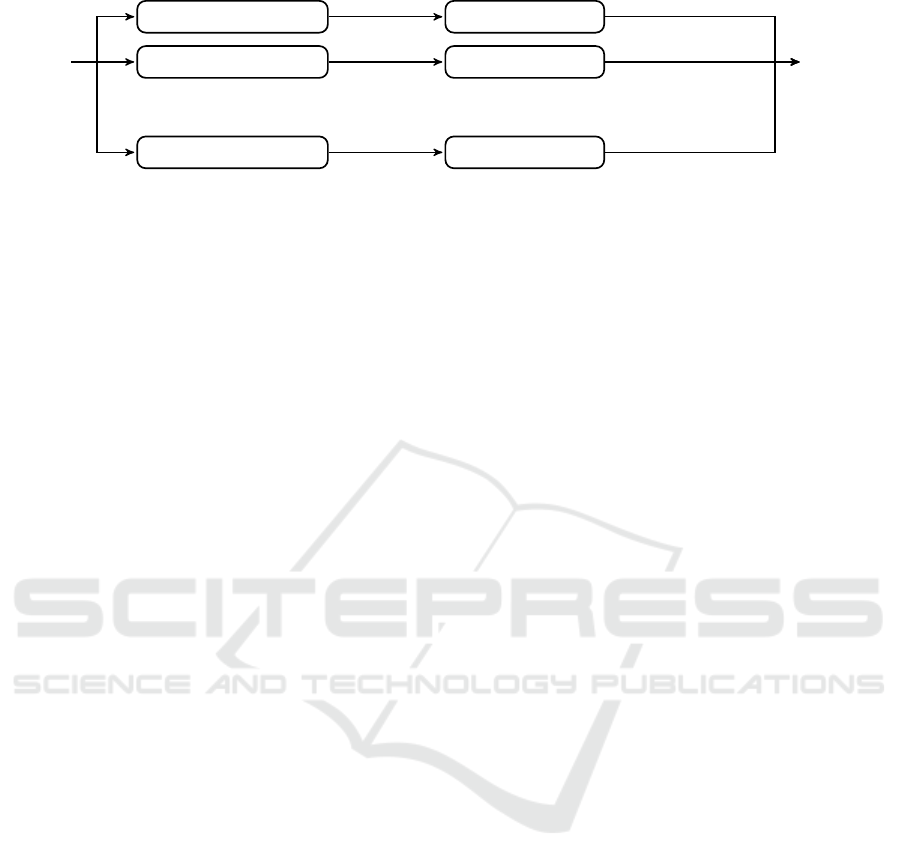
that is used as input to a ﬁnal classiﬁer. An overview

of the process is illustrated in Fig. 2.

In formal terms, let Ω be the set of possible class

labels and D the set of weak classiﬁers considered. A

matrix M of dimensions |D|×|Ω| is computed, which

contains the conﬁdence (represented as probabilities)

that each of the |D| weak classiﬁers gives to the sam-

ple at issue of belonging to each of the |Ω| classes.

That is, M

i j

represents the probability of sample be-

longing to the class Ω

based on the weak classiﬁer

. The matrix can thus be viewed as a new feature

representation (meta-features) that can be used to feed

the ﬁnal classiﬁer rather than using the original fea-

tures. This idea is based on the Decision Templates

proposed by (Kuncheva, 2001). The difference in our

case is that the probabilities are computed from just

one classiﬁer, instead of using many of them.

The construction of this matrix therefore requires

different groups of features to be extracted from the

original image. Each weak classiﬁer is trained for a

particular set of features, thus producing conﬁdence

values that work on the different points of view of

the input data. Note that all weak classiﬁers retrieve

a vector of size |Ω| (probability of the sample of be-

longing to each of the possible classes) independently

of the dimensionality of the input for each of them,

thus allowing to group the results in a single matrix.

However, as the different weak classiﬁers are totally

independent, each one may use different methods or

measures to estimate the probability.

The use of such Conﬁdence Matrix (CM) repre-

Recognition of Handwritten Music Symbols using Meta-features Obtained from Weak Classiﬁers based on Nearest Neighbor

Sample

Feature Extraction 1

Feature Extraction 2

...

Feature Extraction |D|

Weak classiﬁer 1

Weak classiﬁer 2

...

Weak classiﬁer |D|

Conﬁdence

Matrix

(|D| × |Ω|)

Features 1

Features 2

Features |D|

Conﬁdence values 1

Conﬁdence values 2

Conﬁdence values |D|

Figure 2: Graphical scheme of the construction of a Conﬁdence Matrix representation.

sentation entails a set of intrinsic advantages. A ﬁrst

one is that, unlike classical approaches in which the

ﬁnal classiﬁer has the responsibility of discovering

the different points of view of the signal, the ﬁnal

classiﬁer in this matrix representation is already pro-

vided with this segmentation by weak classiﬁers. Fur-

thermore, in contrast to ensemble classiﬁers, this new

scheme avoids the need for deﬁning distinct dissimi-

larity measures or types of weak classiﬁers as features

may be grouped according to their nature, which is of-

ten relatively simple for a user with domain expertise.

From an algorithmic point of view, some addi-

tional advantages are its straightforward implemen-

tation and that the pipeline of the algorithm can be

easily parallelized so that each weak classiﬁer runs at

the same time. Additionally, there may be some sce-

narios in which the CM is not only helpful but also

necessary. For example, when several input features

from the same sample come from different, incompat-

ible structures (eg. trees, strings or feature vectors).

In these cases, scores from weak classiﬁers trained

separately with each kind of structure can be easily

combined within the matrix representation.

Note, however, that this new scheme does not pro-

duce a ﬁnal decision. It merely maps the input fea-

tures into another space (meta-features). This signi-

ﬁes that it is necessary to use an algorithm that em-

ploys the matrix to make a decision using it as a set of

features.

We shall now introduce the different elements

comprising the proposed scheme: the initial features

directly retrieved from the image, the features ob-

tained considering the set of weak classiﬁers, and the

schemes considered for the ﬁnal classiﬁcation stage.

2.1 Groups of Features from Isolated

Music Symbols

Given an input image depicting an isolated music

symbol that has undergone a binarization process, a

preprocessing stage is performed ﬁrst. A morpholog-

ical closing ﬁlter (Serra, 1982) is applied in order to

correct any gaps and spurious points that may have

appeared in the binarization process. In the next step,

.......................................................

................................*.*******..............

...............................************............

.............................***************...........

..........................*******************..........

....................*************************..........

...................****************.....******.........

...................*************.........*****.........

..................*********..*...........*****.........

................**********...............*****.........

..............***********................*****.........

.............**********..................*****.........

.............*********..................******.........

.............*********..................*****..........

..............********.................*****...........

..............*******.................******...........

................*****.................******...........

................*****................******............

................*****...............******.............

................****...............******..............

...............*****.............*******...............

...............*****...........*******.................

..............******.........********..................

..............******........********...................

..............******......*********....................

..............******.....********......................

..............******..**********.......................

..............*****************........................

.............*****************.........................

............*****************..........................

...........*****************...........................

...........*************...............................

...........***********.................................

............*******....................................

............*****......................................

...........******......................................

..........******.......................................

..........*****........................................

.........******........................................

.........*****.........................................

..........****.........................................

...........***.........................................

.......................................................

Figure 3: Example of binary input representing an isolated

handwritten Half Note (

“

the character is located in the image and the region of

interest (ROI) is selected.

Once the image has been preprocessed, the fea-

ture extraction takes place. The image is divided into

a sub-structure of smaller regions in order to extract

local features. The number of sub-regions must be

ﬁxed empirically.

For the sake of clarity in the explanation, let us

consider the input image shown in Fig. 3 as example,

which depicts an isolated Half Note. Three groups of

features are considered for this work:

• Foreground area: a vector with the foreground

area in terms of pixels for each sub-region of the

image is produced (see Fig. 4). Note that, if one

pixel belongs to more than one region it is counted

proportionally within each one.

• Background area: this feature extraction, which is

based on that of (Vellasques et al., 2006), com-

putes four projections (up, down, left, and right)

for each pixel in the image; a counter is set to

zero for each pixel in the image and, when any of

these projections touches the foreground object,

the counter associated to that pixel increases in

ICPRAM 2017 - 6th International Conference on Pattern Recognition Applications and Methods

.........1111111111111111111111111111111111111.........

11111111122222222222222222222222*3*******22222111111111

1111111112222222222222222222222************222111111111

11111111122222222222222222222***************22111111111

11111111122222222222222222*******************2111111111

11111111122222222222*************************2111111111

1111111112222222222****************55555******111111111

1111111112222222222*************555555555*****111111111

111111111222222222*********55*55555555555*****111111111

1111111112222222**********555555555555555*****111111111

11111111122222***********5555555555555555*****111111111

1111111112222***********55555555555555555*****111111111

1111111112222**********555555555555555555*****111111111

1111111112222*********555555555555555555******111111111

1111111112222*********555555555555555555*****2111111111

11111111122223********55555555555555555*****22111111111

11111111122223*******55555555555555555******22111111111

111111111222233******55555555555555555******22111111111

1111111112222333*****5555555555555555******222111111111

1111111112222333*****555555555555555******2222111111111

1111111112222333****555555555555555******22222111111111

111111111222233*****5555555555555*******222222111111111

111111111222233*****55555555555*******22222222111111111

11111111122223******555555555********222222222111111111

11111111122223******55555555********2222222222111111111

11111111122223******555555*********22222222222111111111

11111111122223******55555********2222222222222111111111

11111111122223*******5**********22222222222222111111111

11111111122223*****************222222222222222111111111

1111111112222*****************2222222222222222111111111

111111111222*****************22222222222222222111111111

11111111122*****************222222222222222222111111111

11111111122*************2222222222222222222222111111111

11111111122***********222222222222222222222222111111111

111111111223*******222222222222222222222222222111111111

111111111223******2222222222222222222222222222111111111

11111111122******22222222222222222222222222222111111111

1111111112******222222222222222222222222222222111111111

1111111112*****2222222222222222222222222222222111111111

111111111******2222222222222222222222222222222111111111

111111111*****22222222222222222222222222222222111111111

1111111112****22222222222222222222222222222222111111111

11111111122***22222222222222222222222222222222111111111

.........1111111111111111111111111111111111111.........

266.5 257.0

186.5 274.5

91.0 475.0

20.5 4.5

5.0 0.0

0.0 0.0

101.0 174.5

3.5 0.0

Figure 4: Background features extracted from input consid-

ering 4 sub-regions.

.......................................................

................................1.1111111..............

...............................111111111111............

.............................111111111111111...........

..........................1111111111111111111..........

....................1111111111111111111111111..........

...................1111111111111111.....111111.........

...................1111111111111.........11111.........

..................111111111..1...........11111.........

................1111111111...............11111.........

..............11111111111................11111.........

.............11111111111.................11111.........

.............1111111111..................11111.........

.............111111111..................111111.........

.............111111111..................11111..........

..............11111111.................11111...........

..............1111111.................111111...........

...............111111.................111111...........

................11111................111111............

................11111...............111111.............

................1111...............111111..............

...............11111.............1111111...............

...............11111...........1111111.................

..............111111.........11111111..................

..............111111........11111111...................

..............111111......111111111....................

..............111111.....11111111......................

..............1111111.1111111111.......................

..............11111111111111111........................

.............11111111111111111.........................

............11111111111111111..........................

...........11111111111111111...........................

...........1111111111111...............................

...........11111111111.................................

............1111111....................................

............111111.....................................

...........111111......................................

..........111111.......................................

..........11111........................................

.........111111........................................

.........11111.........................................

..........1111.........................................

...........111.........................................

.......................................................

163.75 207.75

205.50 15.00

Figure 5: Foreground features extracted from input consid-

ering 4 sub-regions.

one unit. This process allows to distinguish four

different categories of background pixels, accor-

ding to their projection values (1, 2, 3, 4). Zero-

valued counters are discarded. An additional cate-

gory with value 5 is added to provide disambigua-

tion information: this value substitutes the value

of 4 if the pixel lies in an isolated background

area. Eventually, the feature vector derived for

each sub-region contains ﬁve descriptors which

depict the proportion of pixel area covered by

each of the projection categories considered. An

example can be seen in Fig. 5.

• Contour area: the contour of the object is encoded

by the links between each pair of 8-neighbor

pixels using 4-chain codes in the manner proposed

by (Oda et al., 2006). These codes are used to ex-

tract four vectors (one for each direction), and the

proportion of pixel area covered by the number of

each code is counted for the different sub-regions

considered. Figure 6 shows an example of this

feature extraction process.

22.5 18.0

35.5 0.0

18.5 25.5

14.0 6.0

12.5 23.0

10.0 0.5

1.0 6.0

1.0 0.0

.......................................................

...............................3333333334..............

..............................2..........34............

............................32.............4...........

.........................332................4..........

...................333332....................1.........

..................2..........................1.........

..................1................3334.......1........

.................2..............332....4......1........

...............32.............32........1.....1........

.............32...........3332..........1.....1........

............2............2..............1.....1........

............1...........2...............1.....1........

............1..........2...............2......1........

............1.........2................1......1........

............1.........1...............2......2.........

............1.........1..............2......2..........

.............1.......2...............1......1..........

.............1.......1..............2.......1..........

..............4......1.............2.......2...........

...............2.....1............2.......2............

..............2.....2...........32.......2.............

..............1.....1.........32........2..............

.............2......1.......32........32...............

.............1......1......2.........2.................

.............1......1....32.........2..................

.............1......1...2..........2...................

.............1.......332.........32....................

.............1..................2......................

............2..................2.......................

...........2..................2........................

..........2..................2.........................

..........1.................2..........................

..........1.............3332...........................

..........1...........32...............................

..........1........332.................................

..........1.......2....................................

..........1......2.....................................

..........1......1.....................................

.........2.......1.....................................

.........1......2......................................

.........1......1......................................

........2......2.......................................

........1......1.......................................

........1.....2........................................

........1.....1........................................

.........4....1........................................

..........3332.........................................

Figure 6: Contour features extracted from input considering

4 sub-regions.

2.2 Meta-features based on Weak

Classiﬁers

As discussed previously, a set of weak classiﬁers with

which to map each group of features onto conﬁdence

values is needed. In this regard, each weak classiﬁer

has been obtained considering a formula based on the

Nearest Neighbor (NN) rule (Cover and Hart, 1967)

given its conceptual simplicity.

Each weak classiﬁer is trained using a leaving-

one-out scheme: each single sample is isolated from

the training set T and the rest are used in combination

with the NN to produce the conﬁdence values. The

formula detailed below is inspired by (P

erez-Cort

et al., 2000). If x is a training sample, then the conﬁ-

dence value for each possible class w ∈ Ω to represent

instance x is based on the following equation:

p(w|x) =

min

∈T

,x6=x

d(x, x

) + ε

(1)

where T

is the training set for w label and ε is a

non-zero value provided to avoid inﬁnity values. In

our experiments, the dissimilarity measure d(·, ·) is

the Euclidean distance. After calculating the proba-

bility for each class, the values are normalized such

that

∑

w∈Ω

p(w|x) = 1.

Once each training sample has been mapped onto

the probability matrix M, the samples can be used in

the test phase.

2.3 Final Classiﬁers

Once the meta-features have been calculated they are

fed into a conventional classiﬁer to compute a class

hypothesis. Given that each of the |D| weak classiﬁers

is retrieving a vector of |Ω| features, two classiﬁcation

paradigms may be considered for this last stage: on

the one hand, we may construct the M matrix by

Recognition of Handwritten Music Symbols using Meta-features Obtained from Weak Classiﬁers based on Nearest Neighbor

grouping all the features from the weak classiﬁers and

then use a single classiﬁcation algorithm; on the other

hand, a meta-classiﬁer which takes as separate inputs

the |D| feature vectors from the weak classiﬁers may

be also considered.

The underlying idea of meta-classiﬁcation is to

solve a labeling problem by combining the decisions

of individual classiﬁers in order to combine them into

a unique ﬁnal decision (late fusion). Thus, the main

reason for considering the aforementioned strategies

for the ﬁnal classiﬁcation stage is to discard the possi-

bility of observing an improvement in the results with

the proposed idea produced by the use of too simple

classiﬁers. In addition, note that our intention in this

work is to check whether the proposed representation

can improve the performance achieved with classical

feature vectors for the precise task of classifying iso-

lated music symbols and not necessarily trying to out-

perform the existing late fusion techniques.

In terms of actual algorithms, we considered

three different classiﬁers for each of the two men-

tioned categories: as of conventional classiﬁers we

considered Nearest Neighbor, Support Vector Ma-

chine, and Multi-Layer Perceptron; in terms of meta-

classiﬁers, we chose Maximum Average Class Prob-

ability, Stacking-C, and Rotation Forest. For all of

them, we have considered the Waikato Environment

for Knowledge Analysis (WEKA) library (Hall et al.,

2009), each one with their default parameterization.

We shall now brieﬂy introduce these schemes.

2.3.1 Nearest Neighbor

The previously introduced Nearest Neighbor (NN)

rule can also be directly used for classiﬁcation. Let

X = (x

, . . . ,x

) be a set of labeled samples and let

∈ X be the sample that minimizes a dissimilarity

measure d(x, x

) to a test point x. The NN rule (Aha

et al., 1991) assigns to x the label associated with x

2.3.2 Support Vector Machines

Support Vector Machine (SVM) is a supervised

learning algorithm developed by Vapnik (Vapnik,

1998). It seeks for a hyperplane which maximizes the

separation (margin) between the hyperplane and the

nearest samples of each class (support vectors). SVM

assumes a binary classiﬁcation problem and thus

needs an extension to tackle multi-class problems. In

this work we shall use the one-vs-one scheme, which

creates an SVM classiﬁer for each pair of classes.

Additionally, as SVM relies on the use of a Kernel

function to deal with non-linearly separable problems,

we shall consider a ﬁrst-order polynomial kernel for

that purpose.

Finally, the training of the SVM considered in this

work is conducted by the Sequential Minimal Opti-

mization (SMO) algorithm (Platt, 1999).

2.3.3 Muti-Layer Percepton

Artiﬁcial Neural Networks is a family of structures

developed in an attempt to mimic the operation of

the nervous system to solve machine learning prob-

lems. The topology of a neural network can be quite

varied. For this work, the common neural network

called Multi-Layer Perceptron (MLP) is used.

2.3.4 Stacking-C

Given that our classiﬁcation scheme is based on the

main idea of Stacking algorithms (i.e., training a

system to classify with the results of other inde-

pendent classiﬁers), we have included this algorithm

to prove the improvement that can be obtained by

means of the use of meta-features. We have selected

one of the most successful algorithms from this fa-

mily: Stacking-C (Seewald, 2002), an extension to

Stacking to accurately address multi-class problems.

2.3.5 Rotation Forest

Rotation Forest (RoF) (Rodriguez et al., 2006) is an

ensemble method that focuses on building accurate

and diverse classiﬁers. It trains a set of decision trees

(forest), each of which uses an independent feature

extraction. RoF makes use of a base classiﬁer to

generate its decision trees. In our work, two alter-

natives will be considered: C4.5 (Quinlan, 1993) (J48

implementation (Hall et al., 2009)) and Random Fo-

rest (RaF) (Breiman, 2001). The ﬁrst alternative is

proposed by the original article, whilst the latter is

considered due to its remarkably good performance

shown in our preliminary experiments.

2.3.6 Maximum Average Class Proﬁle

In contrast to the previous meta-classiﬁers consi-

dered, a decision can be taken by combining the in-

dividual decisions of each weak classiﬁer. In this re-

gard we have considered the Maximum Average Class

Probability (MACP) (Kuncheva, 2004), which labels

the input query with the class that maximizes the ave-

rage of the probabilities given by each of the weak

classiﬁers.

ICPRAM 2017 - 6th International Conference on Pattern Recognition Applications and Methods

100

3 EXPERIMENTS

3.1 Corpus

The HOMUS dataset (Calvo-Zaragoza and Oncina,

2014) of musical symbols will be used in this ex-

perimentation

. This set contains 15200 handwritten

musical symbols from 100 different musicians spread

over 32 of the most common music symbols. It is

important to stress that the corpus was collected en-

couraging the users to write the symbols as natural as

possible, thereby leading to a high variability in the

music notation found within the dataset, as depicted

in Table 1.

3.2 Evaluation

The evaluation of our method consists in comparing

the proposed strategy against conventional classiﬁca-

tion methods. It is also interesting to know whether

results achieved by our proposal are caused by the

group of features selected or by the CM represen-

tation based on weak classiﬁers. Therefore, experi-

ments report the results with and without using the

meta-feature representation considered. In the for-

mer case, both the raw input image (pixel values after

rescaling the binarised image to 20 × 20, to compare

with previous works (Rebelo et al., 2010)) and the set

of features selected is considered.

Table 2 shows the average results in terms of error

rates obtained in the experimentation considering a 4-

fold cross-validation scheme. A ﬁrst remark to point

out is that classiﬁcation results when considering the

raw image exhibit high error rates since almost all

classiﬁers depict error ﬁgures around 25 % and 35 %.

The highest error value can be seen in the MLP classi-

ﬁer as it only properly performs in 25 % of the situa-

tions whereas the best performing algorithm is the

Random Forest ensemble (RoF RaF).

When considering the group of features for enco-

ding the image instead of its raw version, a remar-

kable improvement in the results is observed. Almost

all classiﬁers exhibit a decrease ranging around 10 %

and 15 % in their error rates, being SVM the one

achieving the best classiﬁcation performance. The

only exception to this general improvement is found

in the MLP classiﬁer in which these features do not re-

port an improvement compared to the raw image case,

thus still exhibiting the lowest performance among

the different methods considered.

The dataset is freely available at http://grﬁa.dlsi.

ua.es/homus/

Focusing now on the use of the CM representa-

tion, it can be checked that this representation en-

tails some additional improvements in the results with

respect to the group of features initially considered

for the image. Particularly, the CM representation

reduces the observed error rate in around 5 % to

7 % with respect to the previous representation, be-

ing again SVM the classiﬁer outperforming the rest

with roughly a 10 % of error rate, which represents

a particularly good result given that there are more

than 30 different classes. The NN classiﬁer consti-

tutes the only case for which the use of this represen-

tation does not suppose an improvement in the results.

Lastly, and in spite of exhibiting the highest error rate

for all classiﬁer using the CM set of features, MLP re-

sults undergo a remarkable improvement with respect

to the two previous data representations of close to a

50 % in terms of error rate.

This general improvement in the results when con-

sidering the CM representation for all algorithms (ex-

cept for NN, in which results hardly change) suggests

that the accuracy boost is due to this alternative

feature representation and not to the use of meta-

classiﬁcation schemes rather than simpler metho-

dologies. That is, independently of the classiﬁcation

scheme considered, an improvement is generally ob-

served when the feature representation is based on

CM.

Finally, results obtained with the MACP strategy

also point out that a basic combination of the deci-

sions of each weak classiﬁer instead of using them as

features for a ﬁnal classiﬁcation stage may be enough

for achieving a competitive error rate (around 17 %

for the data considered). More precisely, as it can be

observed, MACP outperforms on average rather com-

plex schemes such as MLP or Stacking-C.

In order to provide consistent conclusions of our

work, these results must be validated objectively

through statistical tests (Demsar, 2006). In this case

we have considered the Wilcoxon rank-sum tests that

allow a pairwise comparison between different clas-

siﬁcation conﬁgurations. Our main intention is to

check whether our approach improves signiﬁcantly

the conventional classiﬁcation scheme consisting of a

set of extracted features plus direct classiﬁcation. To

this end, Table 3 shows the results of this test com-

paring classiﬁcation with the proposed set of meta-

features (CM) against the results obtained consider-

ing the raw input image and the group of features ini-

tially extracted from the image. The signiﬁcance of p

has been established to 0.05. Note that a comparison

between each classiﬁer with CM and the MACP en-

semble is also checked. While we are aware that re-

sults from a 4-fold cross-validation scheme may not

Recognition of Handwritten Music Symbols using Meta-features Obtained from Weak Classiﬁers based on Nearest Neighbor

101

Table 1: Examples of variability in handwritten musical symbols from HOMUS dataset among different musicians.

Label Symbol Musician 1 Musician 2 Musician 3 Musician 4

C-Clef

Eighth Note

Sixteenth

Rest

Table 2: Comparison of the error rate (%) shown by the different classiﬁers considered when the input representation is based

on the raw image, the set of image features or the matrix representation based on weak classiﬁers. The subregion parameter

for the feature extraction has been optimized for each particular classiﬁer. Additionally, the results when considering the

MACP scheme for combining the decisions of each weak classiﬁer is included.

Classiﬁer

Input representation

Raw image Groups of features Conﬁdence Matrix

NN 32.5 19.7 21.0

SVM 32.4 18.6 11.8

MLP 75.2 75.4 24.2

StackingC 33.4 23.2 18.9

RoF J48 35.6 20.8 16.1

RoF RaF 25.1 18.9 15.4

MACP

17.4

be enough for a robust statistical analysis, it allows

depicting the general behavior of the algorithms.

As observed, the use of the CM features entails

a signiﬁcant accuracy improvement over the raw im-

age for all classiﬁers considered. Additionally, when

compared to the initial group of features extracted

from the image, CM also signiﬁcantly outperforms

the results except for the case of the NN classiﬁer,

in which this analysis does not evidence any statis-

tical difference between the use of these two set of

features.

Finally, the statistical comparison between the

MACP combination of single decisions and the use of

a last classiﬁcation stage for the CM features shows

some interesting results. Rotation Forest ensembles

(both RoF J48 and RoF RaF) as well as SVM are able

to signiﬁcantly outperform the MACP strategy. On

the contrary, NN and MLP show a signiﬁcantly worse

performance than the aforementioned decision com-

bination strategy. Lastly, Stacking-C does not show

a statistically relevant difference in performance with

respect to MACP.

4 CONCLUSIONS

The classiﬁcation of handwritten music symbols is a

remarkably useful process in the ﬁeld of Optical Mu-

sic Recognition which turns to be a quite challenging

ICPRAM 2017 - 6th International Conference on Pattern Recognition Applications and Methods

102

Table 3: Results obtained for the statistical signiﬁcance tests comparing the accuracy of the classiﬁer depicted in the row using

CM-based classiﬁcation against the accuracy of the same ﬁnal classiﬁer when considering the raw image and the features from

the ﬁgure (columns). An additional comparison with the MACP ensemble technique is made to assess the performance of

CM against a basic combinations of decisions. Symbols 3, 7 and = state that results achieved by elements in the rows

signiﬁcantly improve, decrease or do not differ respectively to the results by the elements in the columns. Signiﬁcance has

been set to p < 0.05.

CM Ensemble

Raw features Groups of features MACP

3 = 7

SVM

3 3 3

MLP

3 3 7

StackingC

3 3 =

RoF J48

3 3 3

RoF RaF

3 3 3

problem given the variability expected in the musical

symbols.

In this paper we considered an ensemble-based

strategy which consists in extracting heterogeneous

features that are eventually mapped onto a Conﬁdence

Matrix (CM) as a set of posterior probability values

obtained by a group of weak classiﬁers. This ap-

proach enables the features to be transformed into a

new space (meta-features), thus allowing the dimen-

sionality of the data (in our case) to be reduced and a

more meaningful value to be provided in each dimen-

sion. This is expected to help to reduce the error rate

of the ﬁnal classiﬁer.

Our results show that the use of this alternative

space provides signiﬁcant improvements in the results

with respect to the use of image-based features for

most classiﬁers studied. Among the ﬁgures obtained,

Support Vector Machine with the Conﬁdence Matrix

representation yields the best results, which is even-

tually estimated in around 10 % of error rate for the

considered handwritten music symbol data.

Future work considers the inclusion of this pro-

posal in a functional Optical Musical Recognition

system to study its impact in a real-world context.

Additionally, with the intention of still lowering the

error rate obtained, we aim at exploration Convolu-

tional Neural Networks given their reported success

in image processing tasks.

ACKNOWLEDGEMENTS

This work has been supported by the Spanish Ministe-

rio de Educaci

on, Cultura y Deporte through FPU fel-

lowship (AP2012-0939), Vicerrectorado de Investi-

gaci

on, Desarrollo e Innovaci

on de la Universidad de

Alicante through the FPU programme (UAFPU2014–

5883) and the Spanish Ministerio de Econom

ıa y

Competitividad Project TIMuL (No. TIN2013–

48152–C2–1–R supported by UE FEDER funds).

REFERENCES

Aha, D. W., Kibler, D., and Albert, M. K. (1991). Instance-

based learning algorithms. Mach. Learn., 6(1):37–66.

Bainbridge, D. and Bell, T. (2001). The challenge of optical

music recognition. Computers and the Humanities,

35(2):95–121.

Breiman, L. (2001). Random forests. Machine learning,

45(1):5–32.

Burges, C. J. C. (1998). A tutorial on support vector

machines for pattern recognition. Data Mining and

Knowledge Discovery, 2:121–167.

Calvo-Zaragoza, J. and Oncina, J. (2014). Recognition of

pen-based music notation: The HOMUS dataset. In

22nd International Conference on Pattern Recogni-

tion, ICPR 2014, Stockholm, Sweden, August 24-28,

2014, pages 3038–3043.

Cover, T. and Hart, P. (1967). Nearest neighbor pattern clas-

siﬁcation. IEEE Transactions on Information Theory,

13(1):21–27.

Dalitz, C., Droettboom, M., Pranzas, B., and Fujinaga, I.

(2008). A comparative study of staff removal al-

gorithms. IEEE Trans. Pattern Anal. Mach. Intell.,

30(5):753–766.

Demsar, J. (2006). Statistical comparisons of classiﬁers

over multiple data sets. Journal of Machine Learning

Research, 7:1–30.

Duda, R. O. and Hart, P. E. (1973). Pattern Recognition and

Scene Analysis. John Wiley and Sons, New York.

Hall, M., Frank, E., Holmes, G., Pfahringer, B., Reutemann,

P., and Witten, I. H. (2009). The weka data min-

Recognition of Handwritten Music Symbols using Meta-features Obtained from Weak Classiﬁers based on Nearest Neighbor

103

ing software: An update. SIGKDD Explor. Newsl.,

11(1):10–18.

Jain, A. K., Mao, J., and Mohiuddin, K. M. (1996). Artiﬁ-

cial neural networks: A tutorial. Computer, 29(3):31–

44.

Kittler, J., Hatef, M., Duin, R. P. W., and Matas, J. (1998).

On combining classiﬁers. IEEE Trans. on Patt. Anal.

Machine Intelligencet, 20:226–239.

Kuncheva, L. I. (2001). Using measures of similarity and in-

clusion for multiple classiﬁer fusion by decision tem-

plates. Fuzzy sets and systems, 122(3):401–407.

Kuncheva, L. I. (2004). Combining pattern classiﬁers :

methods and algorithms. John Wiley & Sons.

Oda, H., Zhu, B., Tokuno, J., Onuma, M., Kitadai, A., and

Nakagawa, M. (2006). A Compact On-line and Off-

line Combined Recognizer. In Tenth International

Workshop on Frontiers in Handwriting Recogntion,

volume 1, pages 133–138.

erez-Cort

es, J. C., Llobet, R., and Arlandis, J. (2000). Fast

and Accurate Handwritten Character Recognition Us-

ing Approximate Nearest Neighbours Search on Large

Databases. In Ferri, F. J., I

nesta, J. M., Amin, A., and

Pudil, P., editors, Advances in Pattern Recognition,

volume 1876 of Lecture Notes in Computer Science,

pages 767–776, Berlin. Springer-Verlag.

Platt, J. C. (1999). Advances in kernel methods. chapter

Fast training of support vector machines using sequen-

tial minimal optimization, pages 185–208. MIT Press,

Cambridge, MA, USA.

Quinlan, J. R. (1993). C4.5: Programs for machine learn-

ing. Machine Learning.

Rebelo, A., Capela, G., and Cardoso, J. S. (2010). Optical

recognition of music symbols: A comparative study.

Int. J. Doc. Anal. Recognit., 13(1):19–31.

Rebelo, A., Fujinaga, I., Paszkiewicz, F., Marcal, A.,

Guedes, C., and Cardoso, J. (2012). Optical music

recognition: state-of-the-art and open issues. Inter-

national Journal of Multimedia Information Retrieval,

1(3):173–190.

Rico-Juan, J. R. and Calvo-Zaragoza, J. (2015). Improv-

ing classiﬁcation using a conﬁdence matrix based on

weak classiﬁers applied to OCR. Neurocomputing,

151:1354–1361.

Rodriguez, J., Kuncheva, L., and Alonso, C. (2006). Rota-

tion forest: A new classiﬁer ensemble method. IEEE

Transactions on Pattern Analysis and Machine Intel-

ligence, 28(10):1619–1630.

Romero, V., Toselli, A. H., and Vidal, E. (2012). Multi-

modal Interactive Handwritten Text Transcription. Se-

ries in Machine Perception and Artiﬁcial Intelligence

(MPAI). World Scientiﬁc Publishing.

Seewald, A. K. (2002). How to make stacking better and

faster while also taking care of an unknown weak-

ness. In Proceedings of the Nineteenth International

Conference on Machine Learning, ICML ’02, pages

554–561, San Francisco, CA, USA. Morgan Kauf-

mann Publishers Inc.

Serra, J. (1982). Image Analysis and mathematical mor-

phology. Academic Press.

Vapnik, V. N. (1998). Statistical learning theory. Wiley, 1

edition.

Vellasques, E., Oliveira, L., Jr., A. B., Koerich, A., and

Sabourin, R. (2006). Modeling Segmentation Cuts

Using Support Vector Machines. In Tenth Interna-

tional Workshop on Frontiers in Handwriting Recogn-

tion, volume 1, pages 41–46.

ICPRAM 2017 - 6th International Conference on Pattern Recognition Applications and Methods

104