
Domain Adaptation Transfer Learning by SVM Subject to a
Maximum-Mean-Discrepancy-like Constraint
Xiaoyi Chen and R´egis Lengell´e
LM2S, Institut Charles Delaunay, UMR CNRS 6281, University of Technology of Troyes,
12 rue Marie Curie, CS 42060 - 10004, Troyes Cedex, France
{xiaoyi.chen, regis.lengelle}@utt.fr
Keywords:
Transfer Learning, Kernel, SVM, Maximum Mean Discrepancy.
Abstract:
This paper is a contribution to solving the domain adaptation problem where no labeled target data is available.
A new SVM approach is proposed by imposing a zero-valued Maximum Mean Discrepancy-like constraint.
This heuristic allows us to expect a good similarity between source and target data, after projection onto an
efficient subspace of a Reproducing Kernel Hilbert Space. Accordingly, the classifier will perform well on
source and target data. We show that this constraint does not modify the quadratic nature of the optimization
problem encountered in classic SVM, so standard quadratic optimization tools can be used. Experimental
results demonstrate the competitiveness and efficiency of our method.
1 INTRODUCTION
Recently, Transfer Learning has received much at-
tention in the machine learning community. First
formally defined in (Pan and Yang, 2010), the aim
of Transfer Learning is to learn a good-performance
classifier or regressor in a new domain with the help
of previous knowledge issued from different but re-
lated domains; the new domain is designated as tar-
get while domains of previous knowledge are desig-
nated as sources. In this paper, we propose to solve
the transfer learning problem where there is no la-
beled target data available. According to the taxon-
omy given in (Pan and Yang, 2010), our proposed
method belongs to the transductive transfer learning
where the source and the target share the same label
space but differentiate from each other in the feature
space. Marginal, conditional distributions and priors
might differ. This problem is also known as domain
adaptation.
There is a variety of methods for transfer learn-
ing. In this paper, we propose the use of a Support
Vector Machine (SVM) subject to a zero valued Maxi-
mum Mean Discrepancy (MMD)-like constraint. The
choice of a zero-valued MMD as the constraint is
that MMD is a non-parametric measure of the dis-
tance between 2 distributions (Dudley, 2002) and it
can be easily kernelized (Gretton et al., 2012). There-
fore, the combination of MMD and SVM is promis-
ing. SVM is a widely known classification method
used in binary classification. It is well known for
its high generalization ability and the simplicity in
dealing with non-linearly separable data set by using
the kernel trick. Our method keeps these advantages
while performing well in the transfer learning con-
text. As shown in section 3, the optimization problem
remains convex and can be directly implemented us-
ing standard quadratic optimization tools. Adding a
MMD-like constraint is a heuristic that allows us to
expect that source and target data will become similar
in some selected subspace of the feature space. There-
fore, the separating hyperplane found by SVM for
source data can perform well for target data. The ex-
perimental results prove the effectiveness of our idea.
This paper is organized as follows: in section 2,
we give a short summary of related work; then we
present our method in section 3 together with the op-
timization solution to the problem (in section 4); we
prove the effectiveness of the proposed method on
synthetic and real data sets in section 5. Finally, we
conclude this paper and suggest perspectives.
2 RELATED WORK
Because the aim of our work is to perform MMD-like
SVM based transductive transfer learning, we first re-
view the general transductive transfer learning prob-
lem, followed by a presentation of SVM based trans-
fer learning and MMD based transfer learning. Inter-
Chen, X. and Lengellé, R.
Domain Adaptation Transfer Learning by SVM Subject to a Maximum-Mean-Discrepancy-like Constraint.
DOI: 10.5220/0006119900890095
In Proceedings of the 6th International Conference on Pattern Recognition Applications and Methods (ICPRAM 2017), pages 89-95
ISBN: 978-989-758-222-6
Copyright
c
2017 by SCITEPRESS – Science and Technology Publications, Lda. All rights reserved
89

ested readers are referred to (Pan and Yang, 2010) and
(Jiang, 2008) for more general transfer learning and
domain adaptation surveys. For a more recent survey
on domain adaptation, readers are referred to (Patel
et al., 2015)
Transductive transfer learning refers to a shared
label space but different source and target feature
spaces with different marginal and/or conditional dis-
tributions (Pan and Yang, 2010). To take full advan-
tage of source information is the key issue to make the
improvement in learning the target task. When target
labels are not available, typical methods include in-
stance weighting (Huang et al., 2006) with the neces-
sary assumption of the same conditional distributions.
Other authors propose structural corresponding learn-
ing for information retrieval (Blitzer et al., 2007).
SVM based transfer learning adapts the traditional
SVM to the transfer learning context. To the best of
our knowledge, there are five principal kinds of SVM
based transfer learning methods:
• transferring common parameter (w
common
=
w
target
− w
specific
) (Zhang et al., 2009)
• iteratively using SVM to label target domain data
(Bruzzone and Marconcini, 2010)
• reweighting the penalty term of SVM (Liang
et al., 2014)
• adding extra regularization term to standard SVM
(Huang et al., 2012), (Tan et al., 2012)
• SVM by integrating a transformed alignement
constraint combining the knowledge of different
natures (Li et al., 2011)
MMD based transfer learning combines the
MMD, which will be presented later in this paper,
with standard learning method to perform transfer. To
the best of our knowledge, MMD is used as a regular-
ization term of the objective function. The principal
idea is to deal with the trade-off between the classifi-
cation performance of source data and the similarity
of source and target. The interested reader could re-
fer to SVM-based transfer learning classification in
(Quanz and Huan, 2009), multiple kernel learning in
(Ren et al., 2010), multi-task clustering in (Zhang
and Zhou, 2012), maximum margin classification in
(Yang et al., 2012), feature extraction in (Pan et al.,
2011) (Uguroglu and Carbonell, 2011), etc.
3 PRESENTATION OF THE MMD
CONSTRAINED SVM METHOD
In this section, we present our MMD constrained
SVM transfer learning method. We first briefly
review the basic theoretical foundations of MMD and
its kernelized version
3.1 Review of Basic Theoretical
Foundations
3.1.1 Maximum Mean Discrepancy
Maximum Mean Discrepancy (MMD) is a non-
parametric distance measure which can be used to
evaluate the difference between two distributions.
The definition of MMD is:
Definition 1 (Maximum Mean Discrepancy (Fortet
and Mourier, 1953)).
Let F be a class of functions f: X → R and p, q
two Borel probabilistic measures defined on X . The
Maximum Mean Discrepancy (MMD) between p and
q is defined as:
MMD[F , p, q] = sup
f∈F
(E
p
[ f(x)] − E
q
[ f(y)])
As a ”distance measure” between two distribu-
tions, MMD has the following property:
Theorem 1 (Dudley, 1984).
Let (X ,d) be a metric space and p, q two Borel prob-
abilistic measures defined on X , p = q iff E
p
[ f(x)] =
E
q
[ f(y)] for any function f ∈ C(X ), where C(X ) is
the space of continuous bounded functions and x, y
are random variables drawn from distribution p and q
respectively.
Thanks to the works of Smola (Smola, 2006) and
Gretton et al. (Gretton et al., 2012), distributions can
be embedded in a Reproducing Kernel Hilbert Space
(RKHS), where a distribution can be considered as
some mean element of this RKHS (H ):
µ[P
x
] = E
x
[k(x, .)]
(Smola et al., 2007). Accordingly, MMD can be
evaluated as MMD[F , p,q] = kµ
p
− µ
q
k
H
, where µ
r
stands for E
r
[k(x, .)] and k(x, .) is the representation
of x in the RKHS.
As a simple deduction, the squared MMD is:
MMD
2
[F , p, q] = kµ
p
− µ
q
k
2
H
= E
p,p
[k(x, x
′
)] − 2E
p,q
[k(x, y)] + E
q,q
[k(y,y
′
)]
Here, x and x
′
are independent observations drawn
from distribution p, y and y
′
are independent obser-
vations from distribution q, k designates a universal
kernel function (which means that k(x,.) is continu-
ous for all x and the RKHS induced by k is dense in
C(X )).
ICPRAM 2017 - 6th International Conference on Pattern Recognition Applications and Methods
90

Theorem 2 (Steinwart (Steinwart, 2002) and Smola
(Smola, 2006)).
MMD[F , p, q] = 0 iff p = q when F = { f : k fk
H
≤
1} provided that H is universal.
An unbiased estimate of kernelized squared MMD
is proposed in (Serfling, 2009):
\
MMD
2
u
[F ,X,Y] =
1
m(m− 1)
m
∑
i=1
m
∑
j6=i
k(x
i
,x
j
)
+
1
n(n− 1)
n
∑
i=1
n
∑
j6=i
k(y
i
,y
j
) −
2
nm
m
∑
i=1
n
∑
j=1
k(x
i
,y
j
)
where x
i
,i = 1, ... , m and y
i
,i = 1, ... , n are iid exam-
ples drawn from p and q respectively.
SVM aims to find the hyperplane that maximally
separates two classes. The commonly used formula-
tion is:
min
1
2
||w||
2
+C
n
∑
i=1
ε
i
s.t. ε
i
≥ 0
y
i
(w
T
φ(x
i
) + b) ≥ 1− ε
i
∀i = 1, ...,n
where, as usual, w is the hyperplane parameter, ε
i
is
the error term associated to observation i, C is the
trade-off parameter between the margin term and the
classification error, φ(x
i
) is the kernel representation
of x
i
, y
i
is the label of x
i
and b is the bias.
3.2 MMD Constrained SVM Transfer
Learning
We now propose a heuristic to constrain the hyper-
plane that maximizes the margin between the source
classes (and minimizes the corresponding classifica-
tion error) to lie in a subspace where source and tar-
get distributions are as similar as possible. Another
assumption is that the conditional probability distri-
butions of labels are also similar (hypothesis that can-
not be verified because the target labels are supposed
unknown). Accordingly, we can expect the classi-
fier to perform well, both on source and target data.
The heuristic used to maximize the similarity between
source and target is to satisfy the proposed constraint:
< µ
X
s
− µ
X
t
,w >
H
= 0
where µ
X
s
(µ
X
t
) is the sample mean of source (target)
data in H and can be estimated by µ
X
s
=
1
n
s
∑
φ(X
s
)
(µ
X
t
=
1
n
t
∑
φ(X
t
)).
By imposing < µ
X
s
− µ
X
t
,w >
H
= 0, we expect
that source and target data will be similar in H .
The SVM problem can now be formulated as fol-
lows:
min
1
2
||w||
2
+C
n
∑
i=1
ε
i
s.t. < µ
X
s
− µ
X
t
,w >
H
= 0
ε
i
≥ 0
y
i
(w
T
φ(x
i
) + b) ≥ 1− ε
i
∀i = 1, ...,n
(1)
Our approach of using a MMD-like constraint in-
stead of a MMD-regularization-term is to guarantee
the transfer ability. In (Quanz and Huan, 2009),
Quanz and Huan suggest to solve the problem :
min
1
2
||w||
2
+C
∑
n
i=1
ε
i
+ λ|| < µ
X
s
− µ
X
t
,w >
H
||
2
. In
that case, depending on the finite value of the regu-
larization parameter λ, we may sometimes sacrifice
this similarity to achieve a high classification accu-
racy for source only. Furthermore, during the opti-
mization process, their method requires the calcula-
tion of the inverse of a matrix which slows down the
algorithm and causes inaccuracy,while this is avoided
in our work.
4 DUAL FORM OF THE
OPTIMIZATION PROBLEM
In order to solve the above primal problem, we use the
representer theorem (Sch¨olkopf et al., 2001). w, the
optimum solution of Equation 1 in the above section ,
can be expressed as:
w =
n
s
∑
k=1
β
s
k
φ(x
s
k
) +
n
t
∑
l=1
β
t
l
φ(x
t
l
) (2)
where β
s
k
and β
t
l
are the unknowns. Incorporating this
expression into the constraint, we obtain:
< µ
X
s
− µ
X
t
,w >
H
=<
1
n
s
n
s
∑
i=1
φ(x
i
) −
1
n
t
n
t
∑
j=1
φ(x
j
),
n
s
∑
k=1
β
s
k
φ(x
s
k
) +
n
t
∑
l=1
β
t
l
φ(x
t
l
) >
H
=
1
n
s
n
s
∑
k=1
β
s
k
n
s
∑
i=1
< φ(x
i
),φ(x
k
) >
H
−
1
n
t
n
s
∑
k=1
β
s
k
n
t
∑
j=1
< φ(x
j
),φ(x
k
) >
H
+
1
n
s
n
t
∑
l=1
β
t
l
n
s
∑
i=1
< φ(x
i
),φ(x
l
) >
H
−
1
n
t
n
t
∑
l=1
β
t
l
n
t
∑
j=1
< φ(x
j
),φ(x
l
) >
H
= (K
e
1)
T
β
Domain Adaptation Transfer Learning by SVM Subject to a Maximum-Mean-Discrepancy-like Constraint
91

where K =
K
SS
K
TS
K
ST
K
TT
,K
SS
=< φ(x
i
),φ(x
k
) >
H
,
K
TS
=< φ(x
j
),φ(x
k
) >
H
,K
ST
=< φ(x
i
),φ(x
l
) >
H
,
K
TT
=< φ(x
j
),φ(x
l
) >
H
. Here x
i
,x
k
∈ X
s
and x
j
,x
l
∈
X
t
; β = [β
s
,β
t
]
T
and
e
1 = [
1
n
s
,...,
1
n
s
|
{z }
n
s
,−
1
n
t
,..., −
1
n
t
|
{z }
n
t
]
T
.
Incorporating w (2) into ||w||
2
, we have : ||w||
2
=
β
T
Kβ.
We now introduce the Lagrange parameters to solve
this constrained problem:
L = max
α,µ,η
min
β,ε,b
1
2
β
T
Kβ+C
n
s
∑
i=1
ε
i
−
n
s
∑
i=1
α
i
ε
i
−
n
s
∑
i=1
µ
i
[y
i
(β
T
φ(X)φ(x
i
) + b) − 1+ ε
i
] − η(K
e
1
T
β)
After some manipulations, we obtain the dual form:
max
µ,η
n
s
∑
i=1
µ
i
−
1
2
(
n
s
∑
i=1
µ
i
y
i
K
.i
)
T
K
−1
(
n
s
∑
j=1
µ
j
y
j
K
. j
)
−
1
2
η
2
e
1
T
K
T
e
1− η(
n
s
∑
i=1
µ
i
y
i
K
.i
)
T
e
1
s.t. 0 ≤ µ
i
≤ C and
n
s
∑
i=1
µ
i
y
i
= 0
where K
.i
=< φ(X), φ(x
i
) >
H
and X represents the
ensemble of X
s
and X
t
; x
i
is a single point either from
X
s
or X
t
.
As there are two different kinds of Lagrange pa-
rameters µ and η, we eliminate one by first fixing the
value of µ and maximizing only the two latter terms
(related with η) of the Lagrange function. The op-
timal value of η can be expressed as a function of
µ: η = −
(
∑
ns
i=1
µ
i
y
i
K
.i
)
T
e
1
e
1
T
K
T
e
1
. We now obtain the final dual
form of the optimization problem:
max
µ
n
s
∑
i=1
µ
i
−
1
2
(
n
s
∑
i=1
µ
i
y
i
K
.i
)
T
(K
−1
−
e
1
e
1
T
e
1
T
K
T
e
1
)(
n
s
∑
j=1
µ
j
y
j
K
. j
)
s.t. 0 ≤ µ
i
≤ C and
n
s
∑
i=1
µ
i
y
i
= 0.
Let γ
i
denote µ
i
y
i
, the previous problem becomes:
max
γ
γ
T
Y −
1
2
γ
T
(K
SS
−
K
S.
e
1
e
1
T
K
T
S.
e
1
T
K
T
e
1
)γ
s.t.
n
s
∑
i=1
γ
i
= 0 and min(0,Cy
i
) ≤ γ
i
≤ max(0,Cy
i
).
where K
S.
=
∑
n
s
i=1
K
i.
. The matrix K
SS
−
K
S.
e
1
e
1
T
K
T
S.
e
1
T
K
T
e
1
is
the matrix of inner products (in the subspace orthogo-
nal to w) of source data. As stated in (Paulsen, 2009),
if H is a RKHS on X and H
0
∈ H is a closed sub-
space, then H
0
is also a RKHS on X. Therefore, the
matrix K
new
= K
SS
−
K
S.
e
1
e
1
T
K
T
S.
e
1
T
K
T
e
1
is the new Gram matrix
corresponding to the projected kernel, K
new
is positive
semi-definite.
Considering the dual form of the optimization
problem, we can solve it using standard quadratic
programming tools. However, in order to shorten
calculations, we used here an adaptation of the F-
SVC decomposition algorithm proposed in (Tohm´e
and Lengell´e, 2008). Adaptation and implementation
are straightforward.
5 EXPERIMENTS
5.1 Data Sets
Our goal is to improve the classification performance
on target data with the help of related but different
source data.
To illustrate our method on a simple data set,
we first consider some linearly separable data and
we select the linear kernel (which is not univer-
sal so the heuristic should not lead to satisfactory
results). We generate two almost linearly separa-
ble gaussian groups denoted as source-positive and
source-negative. Then we do the same to generate the
target data (there is no label provided for the target
data). An example of this data set is shown in fig. 1.
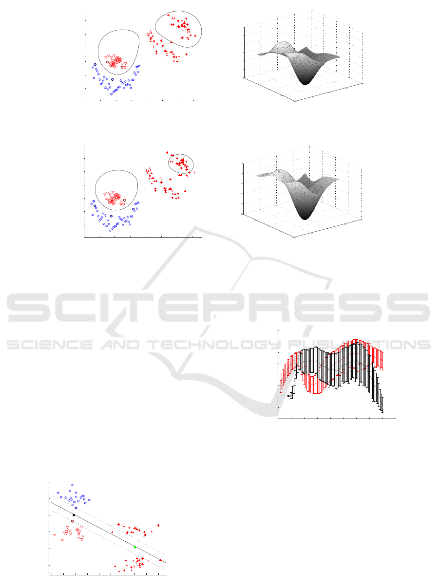
A second, more complicated synthetic data set is
the well-known banana-orange data set. We desig-
nate the banana as the source positive and the orange
as the source negative. We also generate a target data
set which is drawn from a translated and distorted ver-
sion of the distribution of the source data. Here again,
no label information is available for the target (see an
example in fig. 3).
We now use the USPS data set, a famous hand-
written digital number data set. The version used is
composed of training and testing parts, both contain-
ing the image information (16 * 16 pixels) of 10 dif-
ferent numbers. As proposed in (Uguroglu and Car-
bonell, 2011), we choose to separate digits 4 and 7 as
the source classification problem. All the source data
is extracted from the training subset of USPS and is
perfectly labeled. The target classification problem
aims at separating digits 4 and 9 (without the use of
the corresponding labels). All target data is extracted
from the testing subset of the database USPS.
We compare the results we obtained with the
method proposed in (Quanz and Huan, 2009) LM and
also with standard SVM trained only on source data
ICPRAM 2017 - 6th International Conference on Pattern Recognition Applications and Methods
92
−4 −2 0 2 4 6 8 10
0
2
4
6
8
10
(a) Example of a classifier obtained with our
method (for the optimal value of σ)
−5
0
5
10
15
−5
0
5
10
15
−3
−2
−1
0
1
2
3
(b) Decision surface obtained
−4 −2 0 2 4 6 8 10
0
2
4
6
8
10
(c) Example of a classifier obtained with LM
(for the optimal value of σ)
−5
0
5
10
15
−5
0
5
10
15
−4
−2
0
2
4
6
(d) Decision surface (LM)
Figure 3: Results obtained on the banana-orange data set. In 3(a) and 3(c), circles and stars represent the labeled source data
while ”plus” symbols are the unlabeled target data. In 3(b) and 3(d), the decision surfaces are plotted as functions of the input
space coordinates. Thresholding these surfaces at 0 level gives the decision curves corresponding to the classifiers in 3(a) and
3(c), respectively.
(no transfer learning in this case). In (Quanz and
Huan, 2009), LM has been proved superior to other
transfer learning methods so we omit here the com-
parison to other transfer learning methods.
5.2 Experimental Results and Analysis
For a visual comprehension of our SVM-MMD
method, we show in fig. 1 the results obtained on the
first synthetic data set. Stars represent source-positive
data, triangles are source-negative data, crosses are
target data; the two circles are the means of source
−4 −2 0 2 4 6 8 10 12 14
−20
−15
−10
−5
0
5
Figure 1: Linearly separable data set using the linear kernel
(triangles and stars represent the labeled source data, while
”plus” symbols represent the unlabeled target data).
0 0.5 1 1.5 2 2.5 3 3.5 4 4.5
0.4
0.5
0.6
0.7
0.8
0.9
1
1.1
Figure 2: Average performance (good classification rate)
±1 s.d. as a function of the gaussian kernel parameter. Red
line : our method. Black line : LM.
and target data, respectively. As can be seen, the nor-
mal to the obtained discriminant function is orthogo-
nal to ~m
s
− ~m
t
, as expected (for this kernel, the mean
of the original source (target) data coincides with µ
s
(µ
t
).)
For the second synthetic data set (fig. 2), we
show the classification result we obtained compared
to those of LM. We do not compare with standard
SVM on source target data, because obviously stan-
dard SVM will fail here (see fig. 3(a)). Example of
classification results (data sets, discriminant functions
obtained on source and target, decision surfaces) are
shown in fig. 3.
Domain Adaptation Transfer Learning by SVM Subject to a Maximum-Mean-Discrepancy-like Constraint
93
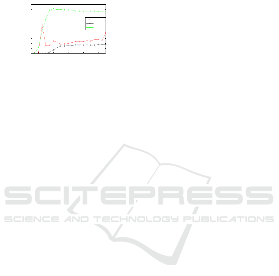
0 1 2 3 4 5 6 7 8 9 10
0.5
0.55
0.6
0.65
0.7
0.75
0.8
0.85
0.9
0.95
1
LM
SVM
SVMMMD
Figure 4: Results (good classification rates) obtained on the
USPS data set as a function of the gaussian kernel parame-
ter.
We independently generate 50 different banana-
orange data sets and show the average performance
(±1 standard deviation) in fig. 2. We conclude that
most of the time our method achieves better results
than LM for a wider range of the kernel parameter
value.
We now show the results obtained on the USPS
data set. As shown in fig. 4, our method provides
higher performance for almost all the kernel parame-
ter values considered.
6 CONCLUSION AND FUTURE
DIRECTIONS
In this paper, we propose a new approach to solve
the domain adaptation problem when no labeled tar-
get data is available. The idea is to perform a pro-
jection of source and target data onto a subspace of a
RKHS where source and target data distributions are
expected to be similar. To do so, we select the sub-
space which ensures nullity of a Maximum Mean Dis-
crepancy based criterion. As source and target data
become similar, the SVM classifier trained on source
data performs well on target data. We have shown that
this additional constraint on the primal optimization
problem does not modify the nature of the dual prob-
lem so that standard quadratic programming tools can
be used. We have applied our method on synthetic
and real data sets and we have shown that our results
compare favorably with Large Margin Transductive
Transfer Learning.
As an important short term development, we must
propose a method to automatically determine an ade-
quate value of the gaussian kernel parameter used in
our paper. We also have to consider multiple kernel
learning. Finally, more complex real data sets are to
be used to benchmark our transfer learning method.
REFERENCES
Blitzer, J., Dredze, M., Pereira, F., et al. (2007). Biogra-
phies, bollywood, boom-boxes and blenders: Domain
adaptation for sentiment classification. In ACL, vol-
ume 7, pages 440–447.
Bruzzone, L. and Marconcini, M. (2010). Domain adapta-
tion problems: A dasvm classification technique and a
circular validation strategy. Pattern Analysis and Ma-
chine Intelligence, IEEE Transactions on, 32(5):770–
787.
Dudley, R. M. (1984). A course on empirical processes. In
Ecole d’´et´e de Probabilit´es de Saint-Flour XII-1982,
pages 1–142. Springer.
Dudley, R. M. (2002). Real analysis and probability, vol-
ume 74. Cambridge University Press.
Fortet, R. and Mourier, E. (1953). Convergence de la
r´epartition empirique vers la r´eparation th´eorique.
Ann. Scient.
´
Ecole Norm. Sup., pages 266–285.
Gretton, A., Borgwardt, K. M., Rasch, M. J., Sch¨olkopf, B.,
and Smola, A. (2012). A kernel two-sample test. J.
Mach. Learn. Res., 13:723–773.
Huang, C.-H., Yeh, Y.-R., and Wang, Y.-C. F. (2012).
Recognizing actions across cameras by exploring the
correlated subspace. In Computer Vision–ECCV
2012. Workshops and Demonstrations, pages 342–
351. Springer.
Huang, J., Gretton, A., Borgwardt, K. M., Sch¨olkopf, B.,
and Smola, A. J. (2006). Correcting sample selection
bias by unlabeled data. In Advances in neural infor-
mation processing systems, pages 601–608.
Jiang, J. (2008). A literature survey on domain adaptation
of statistical classifiers. URL: http://sifaka. cs. uiuc.
edu/jiang4/domainadaptation/survey.
Li, L., Zhou, K., Xue, G.-R., Zha, H., and Yu, Y.
(2011). Video summarization via transferrable struc-
tured learning. In Proceedings of the 20th interna-
tional conference on World wide web, pages 287–296.
ACM.
Liang, F., Tang, S., Zhang, Y., Xu, Z., and Li, J. (2014).
Pedestrian detection based on sparse coding and
transfer learning. Machine Vision and Applications,
25(7):1697–1709.
Pan, S. J., Tsang, I. W., Kwok, J. T., and Yang, Q. (2011).
Domain adaptation via transfer component analysis.
Neural Networks, IEEE Transactions on, 22(2):199–
210.
Pan, S. J. and Yang, Q. (2010). A survey on transfer learn-
ing. Knowledge and Data Engineering, IEEE Trans-
actions on, 22(10):1345–1359.
Patel, V. M., Gopalan, R., Li, R., and Chellappa, R. (2015).
Visual domain adaptation: A survey of recent ad-
vances. IEEE signal processing magazine, 32(3):53–
69.
Paulsen, V. I. (2009). An introduction to the theory of re-
producing kernel hilbert spaces. Lecture Notes.
Quanz, B. and Huan, J. (2009). Large margin transductive
transfer learning. In Proceedings of the 18th ACM
conference on Information and knowledge manage-
ment, pages 1327–1336. ACM.
ICPRAM 2017 - 6th International Conference on Pattern Recognition Applications and Methods
94

Ren, J., Liang, Z., and Hu, S. (2010). Multiple kernel learn-
ing improved by mmd. In Advanced Data Mining and
Applications, pages 63–74. Springer.
Sch¨olkopf, B., Herbrich, R., and Smola, A. J. (2001). A
generalized representer theorem. In Computational
learning theory, pages 416–426. Springer.
Serfling, R. J. (2009). Approximation theorems of mathe-
matical statistics, volume 162. John Wiley & Sons.
Smola, A. (2006). Maximum mean discrepancy. In 13th
International Conference, ICONIP 2006, Hong Kong,
China, October 3-6, 2006: Proceedings.
Smola, A., Gretton, A., Song, L., and Sch¨olkopf, B. (2007).
A hilbert space embedding for distributions. In Algo-
rithmic Learning Theory, pages 13–31. Springer.
Steinwart, I. (2002). On the influence of the kernel on the
consistency of support vector machines. The Journal
of Machine Learning Research, 2:67–93.
Tan, Q., Deng, H., and Yang, P. (2012). Kernel mean match-
ing with a large margin. In Advanced Data Mining and
Applications, pages 223–234. Springer.
Tohm´e, M. and Lengell´e, R. (2008). F-svc: A simple and
fast training algorithm soft margin support vector clas-
sification. In Machine Learning for Signal Processing,
2008. MLSP 2008. IEEE Workshop on, pages 339–
344. IEEE.
Uguroglu, S. and Carbonell, J. (2011). Feature selec-
tion for transfer learning. In Machine Learning and
Knowledge Discovery in Databases, pages 430–442.
Springer.
Yang, S., Lin, M., Hou, C., Zhang, C., and Wu, Y. (2012). A
general framework for transfer sparse subspace learn-
ing. Neural Computing and Applications, 21(7):1801–
1817.
Zhang, P., Zhu, X., and Guo, L. (2009). Mining data streams
with labeled and unlabeled training examples. In Data
Mining, 2009. ICDM’09. Ninth IEEE International
Conference on, pages 627–636. IEEE.
Zhang, Z. and Zhou, J. (2012). Multi-task clustering via
domain adaptation. Pattern Recognition, 45(1):465–
473.
Domain Adaptation Transfer Learning by SVM Subject to a Maximum-Mean-Discrepancy-like Constraint
95
