
A General Physical-topological Framework using Rule-based Language
for Physical Simulation
Fatma Ben Salah, Hakim Belhaouari, Agn
`
es Arnould and Philippe Meseure
University of Poitiers, Xlim Lab, UMR CNRS 7252, Futuroscope, France
Keywords:
Physical Animation, Topologically-based Simulation, Rule-based Language, Prototyping.
Abstract:
This paper presents a robust framework that combines a topological model (a generalized map or G-map) and
a physical one to simulate deformable objects. The framework is general since it allows a general simulation of
deformations (1) in different dimensions (2D or 3D), (2) with different types of meshes (triangular, rectangular,
tetrahedral, hexahedral, and combinations of them...) and (3) physical models (mass/spring, linear FEM,
co-rotational, mass/tensor). Any mechanical information is stored in the topological model and is used in
combination with the neighboring relations to compute the equation of motions. To design this model, we
have used JERBOA, a rule-based language relying on graph transformations to handle G-maps. This tool has
been helpful to build and test different physical models in a little time.
1 INTRODUCTION
Physically-based simulation have a great importance
for various computer graphics applications such as
virtual reality, simulation of natural phenomena and
video games. Since the early approaches of Ter-
zopoulos et al. on simulating deformable objects
(Terzopoulos et al., 1987), several models have fo-
cused on simulating realistic behavior of deformable
objects. These models rely on discrete mechan-
ics (mass/spring systems (Provot, 1995)) or continu-
ous mechanics (Finite Element Method (O’Brien and
Hodgins, 1999)), mass/tensor systems (Cotin et al.,
2000), Finite Differences (Terzopoulos et al., 1987)).
Physical models can undergo topological modi-
fications whereas they are based on a rudimentary
topological structure. This usually implies heavy pro-
cesses to ensure that the mesh remains manifold (For-
est et al., 2005). Yet, it is possible to preserve the
manifold property of a mesh by using more robust and
appropriate topological models (Damiand and Lien-
hardt, 2014). The consistency is therefore guaranteed
after topological modifications.
Meseure et al. (Meseure et al., 2010) proposed
to combine a physical model with a topological
one. Their approach is specific to tetrahedral meshes
and mass/spring systems. Thereafter, Fl
´
echon et al.
(Fl
´
echon et al., 2013) extend the use of topological
models to simulate hexahedral (3D) or rectangular
(2D) meshes with mass/spring systems. These ap-
proaches show the effectiveness of using a topologi-
cal model in physically-based animation, particularly
for simulating transformations such as tearing, cut-
tings, etc. However, their solution under-exploit the
capabilities of the topological model to embed any
kind of information. For instance, shear springs are
stored in an additional structure which appears re-
dundant with the topological model (and can poten-
tially result in an inconsistent model association). Re-
cently, Golec et al. (Golec et al., 2015) have proposed
a generic approach to simulate both tetrahedral and
hexahedral meshes using Mass/spring or Mass/tensor
physical models. Their method unfortunately still re-
quires an additional structure to store shear springs
and tensors. This structure includes topological infor-
mation that must be kept consistent with the topolog-
ical model. This is a real issue in case of complex
topological transformations.
This paper proposes several contributions:
• formalization of the physical modeling and ani-
mation of deformable meshed objects using an ap-
propriate topological model (namely generalized
maps or G-maps),
• generalization of the modeling and the behavior
computation with respect to (1) the dimension, (2)
the type of mesh elements and (3) the constitutive
laws,
• fast prototyping using a formal approach based on
rules of graph transformations.
220
Ben Salah F., Belhaouari H., Arnould A. and Meseure P.
A General Physical-topological Framework using Rule-based Language for Physical Simulation.
DOI: 10.5220/0006119802200227
In Proceedings of the 12th International Joint Conference on Computer Vision, Imaging and Computer Graphics Theory and Applications (VISIGRAPP 2017), pages 220-227
ISBN: 978-989-758-224-0
Copyright
c
2017 by SCITEPRESS – Science and Technology Publications, Lda. All rights reserved

It is organized as follows. Section 2 presents the
related work. In Section 3, the main basis of proto-
typing with a rule-based language using the JERBOA
software (Belhaouari et al., 2014) is detailed. In Sec-
tion 4, the physical simulation of 2D and 3D objects
with different types of meshes and physical models
using rule-based language are described. Finally, im-
plementation details are given in Section 5.
2 PREVIOUS WORK
Several previous studies have shown the advantages
of using a topological model for simulation. Meseure
et al. (Meseure et al., 2010) use G-maps to simu-
late the deformation and the topological changes of
soft bodies. Their approach is restricted to tetrahe-
dral meshes and mass/spring systems. Moreover, they
have used only stretching springs, associated to edges.
Nevertheless, due to the G-maps engine used, they re-
quired external arrays to allow a fast access to cells
(vertices, edges, volumes...). These arrays must be
updated after any topological change.
Fl
´
echon et al. (Fl
´
echon et al., 2013) have used a
derivation of combinatorial maps, namely 3D Linear
Cell Complex (LCC) as a topological model to sim-
ulate mass/spring systems based on 2D rectangular
and 3D hexahedral meshes. In this model, stretch-
ing springs are also associated to edges. Unfortu-
nately, shear springs (placed along diagonals of each
element) require an external structure. Golec et al.
(Golec et al., 2015) extend this model to allow the
simulation of 3D tetrahedral and hexahedral meshes
using not only mass/spring but also mass/tensor mod-
els. They claim not to rely on any additional struc-
tures but each face/volume is associated with an array
of darts that allow the numbering of each vertex. Ac-
tually, this array implicitly includes neighboring rela-
tionships so appears as redundant with the LCC.
The real weakness of all these approaches is the
use of external structures to store information re-
quired by the simulation. After a topological mod-
ification, the external structure can be rebuilt from
scratch or be modified incrementally. The first so-
lution guarantees correctness but is costly, while the
second is a tedious process that can lead to inconsis-
tencies. On the contrary, maps ensure their own con-
sistency using constraints that can easily be verified.
It seems that the limitation of element types in
(Meseure et al., 2010) and the use of external struc-
tures in (Fl
´
echon et al., 2013) and (Golec et al.,
2015) is due to an unsuitable modeling of interac-
tions. Indeed, these approaches search for topolog-
ical elements that could support both the origin of
the forces (e.g. a link between two particles) and
the vertices associated with the concerned particles.
Concerning stretching springs, the solution is simple
and immediate, since these topological elements are
edges of the mesh. But the other kinds of springs
do not directly correspond to topological elements
(for instance, diagonals of faces). We therefore pro-
pose a new paradigm to model springs and other me-
chanical components in general, that could be called
“topology-based force field”. Force modeling pro-
cess should focus only on the origin of each force and
store the mechanical parameters on related topologi-
cal elements. Thus, if these elements are modified by
topological modifications, the resulting forces should
be automatically altered. The (two or more) involved
particles should therefore be identified from the stor-
age place, while computing interaction forces.
To sum up, our method overcomes the limitation
of the approaches listed above as it proposes:
• a framework with multi-physical, multidimen-
sional and multi-element simulation;
• a new paradigm to model interactions, by both
considering their physical origin and identifying
the (two or more) involved particles;
• a storage for all the mechanical information in the
topological model (no other additional structure is
necessary).
To simulate deformable bodies using a physical
model and a topological one, a rule-based language
is used which exploits graph transformations for pro-
totyping. This language offers the opportunity to test
the capability of our model to simulate different types
of meshes in different dimensions with different phys-
ical models and different properties (homogeneity,
isotropy) in a little time. Note that a lot of languages
are dedicated to physical modeling, such as (Kjolstad
et al., 2016) among others. These languages often
propose to describe the simulated objects, including
their topology, but contrary to our approach, they do
not aim at programming the simulation itself nor do
they allow the design of new interactions.
3 PROTOTYPING USING RULE
BASED-LANGUAGE
The JERBOA rule-based language (Belhaouari et al.,
2014) is dedicated to geometric modeling. It is based
on the topological model of G-maps (Damiand and
Lienhardt, 2014). The representation of an object us-
ing a G-map is defined from its successive subdivi-
sion into topological cells (vertices, edges, faces, vol-
umes, etc.) and appears as a graph (Figure 1b). The
A General Physical-topological Framework using Rule-based Language for Physical Simulation
221

nodes of this graph are called darts. Arcs represent
the adjacency relationships between cells and are la-
beled by their dimension. In the following figures,
black arcs stand for 0-dimensional, red dotted arcs for
1-dimensional and blue double arcs for 2-dimensional
links.
A
B
C
D
E
(a)
d
b
c
a
m
n
l
j
k
i
g
h
e
f
A
A
B
B
C
C
C
C
B
B
D
D
E
E
(b)
d
b
c
a
m
n
l
j
k
i
g
h
e
f
(c)
d
b
c
a
m
n
l
j
k
i
g
h
e
f
(d)
d
b
c
a
m
n
l
j
k
i
g
h
e
f
(e)
Figure 1: Decomposition of a 2D object and examples of
orbits: (a) Object 2D, (b) G-map(connected component),
(c) Vertex, (d) face and (e) half edge.
Topological cells (i.e. vertices, edges, faces, vol-
umes) of an object are defined by sub-graphs called
orbits. Figure 1 represents some orbits which corre-
spond to cells of the object presented in Figure 1a.
For example, vertex B of Figure 1a is defined by the
sub-graph reachable from dart e using 1- and 2-links
(that is, darts c, e, g, i and the links that connect them),
noted orbit h1, 2i(e) (Figure 1c). Similarly, edge BC
is the orbit h0, 2i(e) and face ABC is the orbit h0, 1i(e)
(see Figure 1d). We should note that the concept of
orbit is not limited to cells and may identify less com-
mon entities, such as half-edges (Figure 1e), or con-
nected components (Figure 1b).
To model an object, the topological structure of G-
maps must be complemented by additional (geomet-
ric, colorimetric, mechanical...) information called
embeddings. These data are attached to darts. For
example, in Figure 1b, darts carry geometrical points
(A, B, C, D and E) and colors (blue and yellow). Each
embedding is characterized by the type of informa-
tion (here a 2D point and a color) and the support or-
bit (here orbit h1, 2i for vertex information and h0, 1i
for face information), but we can also associate infor-
mation to any type of orbits like corner of face h1i.
Besides, as shown in Figure 1b, all darts of a support
orbit should share the same embedding.
A rule created with JERBOA has the form L → R,
where L (left part) is a sub-graph to be matched for
the rule to apply and R (right part) a modification of
this sub-graph, that includes expressions of embed-
ding changes. JERBOA’s rule editor automatically
verifies and ensures the object consistency preserva-
tion. Besides, it allows a fast prototyping of geometric
operations (some examples are given in Section 5).
4 RULE-BASED PHYSICAL
SIMULATION
The modeling process is based on a 2D or 3D mesh
which represents the structure of the object. It is mod-
eled by a G-map, in which mechanical information is
embedded. As stated in previous work, a correct em-
bedding must be selected, that is, the most adapted
topological place with respect to the physical origin
of each property must be found. These properties
include mass, ambient viscosity, etc. that relate to
the physical model (studied in the next subsection) as
well as any interaction model, whether it is discrete or
continuous (studied in the two following subsections).
The same process is always followed: (1) find the
most adapted topological place to embed mechanical
information, (2) from this place, define the adjacency
relations to follow to find on which vertices/particles
the force applies and (3) store the computed force in
adapted sub-orbits of these vertices (for instance, cor-
ner orbit h1i or extremity of edge h2, 3i).
Based on this modeling, the simulation loop pro-
ceeds this way: (1) walk through all the orbits
that embed interaction data and compute the applied
forces, (2) walk through all the vertices and for each
one, collect forces stored in its sub-orbits and com-
pute the sum of forces applied to its particle and (3)
integrate the equation of motion to find new velocity
and positions of each particle.
4.1 Physical Model
The used simulation loop is the same for all physical
models. This implies that every particle has a mass, as
well as an acceleration, a velocity and a position that
must be computed at each time step. These mechani-
cal properties have to be stored in the most appropri-
ate orbit. When the properties are related to a given
cell, the orbit is found immediately. For instance, ac-
celeration, position and velocity of a particle which
are stored on its corresponding vertex (orbit h1, 2, 3i).
Considering mass, several solutions exist and
ought to be discussed. Considering its physical ori-
gin, mass is supposed uniformly distributed over the
surface or the volume of an homogeneous object. On
the one hand, it seems natural to associate mass to
the faces or volumes of the mesh. On the other hand,
only models where mass is concentrated on particles
each surrounding face/volume contributes provide a
vertex with a mass) are considered so mass is stored
in vertices in previous models (the mass of a parti-
cle is the sum of the contributions of each surround-
ing face/volume). As a compromise, the contribution
of a face or a volume to each of its vertex is explic-
GRAPP 2017 - International Conference on Computer Graphics Theory and Applications
222
itly stored in our model. A face distributes its mass
(evenly of not) to all its vertices, that is its sub-orbits
h1i (known as “face corner”). The same way, a vol-
ume distributes mass to its sub-orbits h1, 2i (known
as “volume corner”). In both cases. Now the physi-
cal properties are defined, the interaction model that
is applied to animate is presented in the following sec-
tion.
4.2 Springs Model
Provot proposed three different types of springs,
to control respectively stretching, shear and bend-
ing (Provot, 1995). This approach can be extended
for 3D, where stretch springs correspond to edges of
the mesh, and shear springs appear on diagonal of non
triangular faces and/or non tetrahedral volumes.
As explained earlier, the process consists in find-
ing the right orbit to embed spring information (stiff-
ness, rest-length and possibly damping), defining a
sub-graph to find the vertices implied in the interac-
tion, computing it, and finally storing the computed
forces in appropriate sub-orbits of these vertices. The
sub-orbits where forces are stored can be found eas-
ily: The method always chooses the largest orbit in-
cluded in the intersection of the sub-graph used to find
concerned vertices (blue graph in following figures of
this section) and the vertex orbit itself (orbit h1, 2i in
2D and h1, 2, 3i in 3D, shown in red). It must be noted
that it is delicate to find the right sub-graph for each
type of springs since it must be chosen as generic as
possible, so that it can be applied, if desired, on all
types of faces (triangles, quads or others). Below,
each type of spring is detailed.
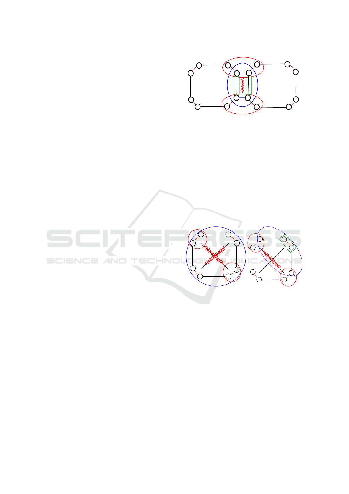
4.2.1 Stretch Springs
Stretch springs connect two particles placed on ver-
tices that are linked by an edge. In 2D, it seems conve-
nient to associate spring information with edge orbits
(h0, 2i) (as proposed in previous approaches). How-
ever, when an edge is adjacent to two faces, each face
provides the edge with strength against stretching that
can be represented as a spring. So, an embedding is
created for any elementary spring (green sub-graph)
associated to orbits h0i (face edges) as shown in Fig-
ure 2 and all these springs are summed for force com-
putation. This gives the sub-graph shown in blue.
In Figure 2, the particles influenced by a stretch
spring are the extremities of the support edge (shown
in red). Forces are computed and stored in a sub-orbit
of each vertex corresponding to the edge, that is h2i.
Here, faces are represented as a quad, but could in-
clude any number of vertices. This approach can be
directly applied for 3D.
2
2
0
0
0
0
0
0
0
0
1
1
1
1
1
1
1
1
Figure 2: Force applied by stretch springs.
4.2.2 Shear Springs
Shear springs are supported by diagonals of a face,
that is, segments that do not correspond to an orbit.
Two main motivations can be considered to include
shear springs: (1) because the face has to maintain its
shape, so produces forces between each couple of op-
posite vertices or (2) because the angles of each cor-
ner of the face must be preserved, so a force must be
applied to the non-connected extremities of any two
adjacent edges. Since mechanical properties can be
chosen freely for each couple of edges, this last ap-
proach is qualified as “anisotropic”.
0
0
0
0
1
1
1
1
(a) Isotropic case
1
11
1
1
0
0
0
0
(b) Anisotropic case
Figure 3: Force applied by shear springs.
In the isotropic model, a rectangular mesh must be
used, since the same stiffness and rest-length is em-
bedded in the face (h0, 1i) for both diagonals. The op-
posite vertices can be found by just walking through
the face, so the face orbit h0, 1i is the sub-graph
needed to find vertices. Computed forces are stored
in the intersection between the sub-graph and the ver-
tex orbits, that is corners of the face (h1i).
In the anisotropic model, elements can be of any
shape or even any topology. The mechanical proper-
ties of a shear spring is stored in orbits h1i that corre-
sponds to the articulation (the angle) between the two
connected edges (shown in green). Since the inter-
section between the two articulated edges (blue sub-
graph) and their non-connected extremities (shown in
red) reduces to single darts, forces are stored in dart
orbits hi, as shown in Figure 3b. Note that this solu-
A General Physical-topological Framework using Rule-based Language for Physical Simulation
223
tion is compatible with triangles (although not useful,
as a stretching spring already binds the same vertices).
In 3D, if shear springs are placed on the diagonals
of hexahedra’ faces, the same embeddings as in 2D
still apply. If shear springs are put on the diagonals
of a hexahedron, a new embedding is associated with
its volume orbit (h0, 1, 2i) and controls four similar
springs. Note that, in this case, volumes should be
rectangular cuboids. Here, computed forces are put in
“corners” of volumes, that is orbits h1, 2i.
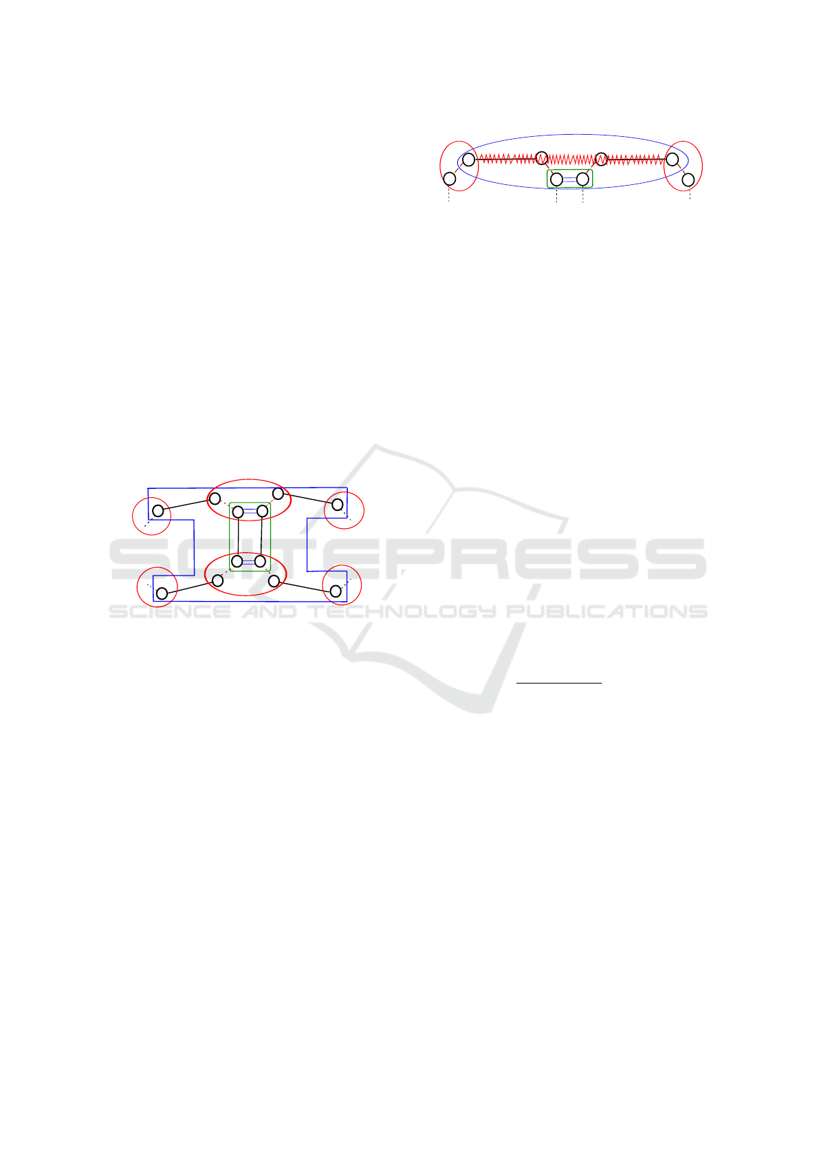
4.2.3 Bending Springs
Considering that bending must be handled by control-
ling the angle between any two adjacent faces, an-
gular springs have been proposed to control bending
((Grinspun et al., 2003), among others), by constrain-
ing the angle between faces supported by the com-
mon edge of two adjacent faces. This angular spring
can be stored in edge orbits h0, 2i (green sub-graph in
Figure 4).
F
C
F
E
FF
D
A
0
0
0
2
2
F
B
B
F
A
C
F
D
F
F
E
0 0
Figure 4: Force applied by an angular spring.
As shown in Figure 4, vertices of faces that are
extremities of edges 1-linked to the articulation edge
must be found (A, B, C, D, E and F) via an appro-
priate sub-graph (in blue), since they must undergo
bending forces. Once calculated, these forces are
stored in orbits dart hi (directly in the dart). Note that
the chosen sub-graph is compatible with any type of
faces, since the links between vertices C and E on
the one hand, and D and F on the other hand, are
not specified in the sub-graph. These vertices can be
the merged (triangles), linked by an edge (quad), or
linked by several edges (other types). Mixed meshes
with different types of faces can be used as well.
To control bending, Provot introduced springs
that connect second-neighbor vertices (Provot, 1995).
These links control the angle between two edges both
connected, via a vertex, to an edge shared by two
faces. This remark gives the sub-graph, represented
in blue in Figure 5. It seems convenient to embed
such spring into the orbit h2i, corresponding to the
common edge and the articulation vertex at once (in
green).
1
1
2
1
1
Figure 5: Force applied by a Provot’s spring.
Computed forces are stored in dart orbit hi. For
the same reason as above, this modeling is compatible
with triangles, even if two orbits h2i link the same
couple of vertices. Mixed meshes can benefit from
these springs as well.
Angular or Provot’s springs aim at simulating the
same effect but their implementations are different.
Thus, both of them are proposed in our model, be-
cause provot’s approach is more efficient in the case
of a rectangular and triangular mesh, while the angu-
lar approach can potentially be generalized to other
types of faces.
4.2.4 Force Computation
Once the vertices linked by a spring are identified, the
force exerted by particle i on particle j is computed
according to:
F
ij
=
−k
i j
kx
j
− x
i
k − l
i j
− λ
i j
v
j
− v
i
· u
ij
u
ij
(1)
where k
i j
is the stiffness, l
i j
the rest length, λ
i j
the
damping coefficient, u
ij
the unitary vector from i to j,
x the position and v the velocity of each particle.
To compute forces applied by angular springs on
edge i, a formula quite similar to Grinspun et al.’s
one (Grinspun et al., 2003) but simplified and ex-
tended to quads, is used for each involved vertex:
F
M
= ±
k
i
× θ
2 × ku × AMk
2
× (u × AM) (2)
with θ is the angle between normals of the two faces
(defined by the edge and the center of the quad), k the
angular stiffness, u the unitary vector of the edge, A
any vertex on the edge and M the vertex where the
force is applied. When a vertex undergoes a force,
the opposite of this force must distributed to vertices
of the edge. Here, we adapt the method to quads by
considering that F
A
= −F
C
− F
D
, (and similarly for
F
B
) in figure 4.
The chosen embeddings in G-maps allow the
modeling of different types of meshes including
mixed ones, in 2D and 3D using the same embed-
dings. However, some constructions, even if cor-
rectly simulated by our system, are not recommended.
For instance, if shear springs are used in triangular
or tetrahedral meshes, they only provide the element
with more stretching so should be omitted. Further-
more, bending springs are, to our knowledge, rarely
GRAPP 2017 - International Conference on Computer Graphics Theory and Applications
224
used in 3D (in practice, they control dihedral angles
of volumes which is rather redundant with stretching
springs).
4.3 Continuous Mechanics Approaches
In this section, the modeling of continuous mechan-
ics is discussed. The same strategy already done with
mass/spring system is applied.
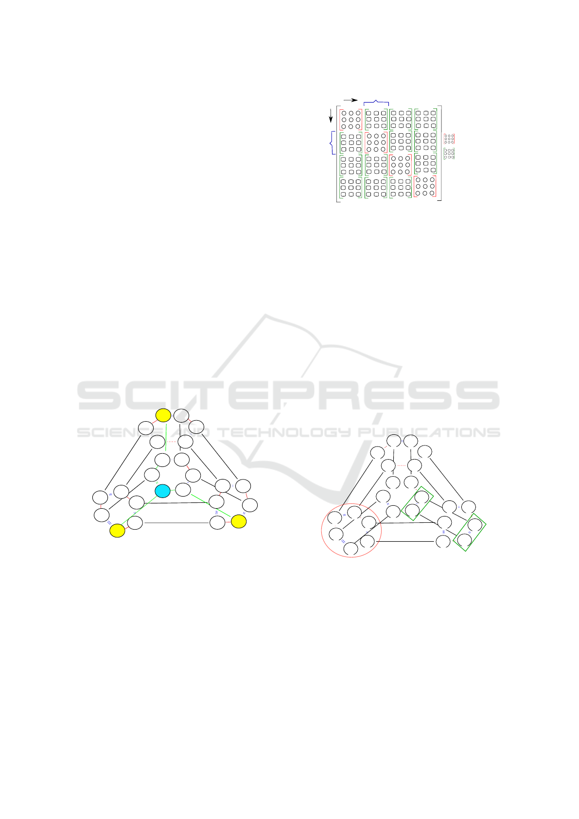
4.3.1 Linear FEM
FEM use a tessellation of an object into a finite num-
ber of elements. In the following, tetrahedra are used.
Each tetrahedron is characterized by a 12x12 stiffness
matrix K (see (O’Brien and Hodgins, 1999)).
Matrix K is computed in a preliminary phase for
each tetrahedron and is embedded into volume or-
bits h0, 1, 2i. Nevertheless, this matrix depends upon
a given order of vertices (positive orientation of the
tetrahedron’s volume) that must be stored in the struc-
ture. Here, we propose to tag only one dart as “fist-
dart” for each volume. As shown in Figure 6, the ver-
tex that owns this dart in its orbit is vertex 1. From
this dart and following the adjacency relations of the
G-maps in a given order, the number of other vertices
is recovered.
1
1
2
1
2
1
2
2
2
2
1
1
1
2
1
2
1
2
0
0
0
0
0
0
2
1
2
1
2
1
α0
α0
α0
α0
α0
<>
<>
<>
<>
<>
<>
<>
<>
<>
<>
<>
<>
<>
<>
<>
<>
<>
<>
<>
<>
<>
<>
1
2
3
4
0
0
First_dart
<>
Figure 6: Numbering of vertices.
At each time step and for each tetrahedron, forces
must be computed as:
f = −Ku (3)
where f includes the forces of all vertices of the tetra-
hedron, and u represents their displacements. Forces
computed are stored in the corresponding “corner” of
the tetrahedron (orbit h1, 2i).
For hexahedra, the approach remains the same,
only the information to embed changes. However,
modeling with FEM using linear elasticity can sim-
ulate only small displacements. To allow rotation
Vertex tensor
Edge tensor
K1,2
j
Kj,i
i
Ki,j =
K2,1
t
Figure 7: Decomposition of a stiffness matrix.
of objects, the Co-rotational method has been im-
plemented using a QR decomposition (Nesme et al.,
2005). The embeddings remain the same, only force
computations slightly differ. This method was also
used to implement 2D FEM for triangular meshes (Et-
zmuss et al., 2003).
4.3.2 Linear Mass/Tensor
In this section, it is shown that our model is well
adapted to the mass/tensor approach as proposed by
(Cotin et al., 2000). This method considers the 12x12
stiffness matrix computed using linear FEM, but de-
composes it into sixteen 3x3 matrices K
ij
. Such a de-
composition is shown in Figure 7. Diagonal matri-
ces (red) show the influence of the displacement of a
vertex on itself. The other matrices (green) show the
influence of any vertex of a tetrahedron on the others.
1
1
2
1
2
1
2
2
2
2
1
1
1
2
1
2
1
2
0
0
0
0
0
0
2
1
2
1
2
1
α0
α0
α0
α0
α0
<>
n44
<>
n13
<>
n25
<>
n33
<>
n45
<>
n24
<>
n21
<>
n26
<>
n23
<>
n22
<>
n43
<>
n46
<>
n41
<>
n42
<>
n34
<>
n35
<>
n36
<>
n31
<>
n32
<>
n14
<>
n15
<>
n16
<>
n11
<>
n12
Tensor
Vertex
Tensor
Vertex
Tensor
edge
Tensor
edge
Tensor
edge
Tensor
edge
Tensor
Vertex
Tensor
Vertex
Tensor
Vertex
Tensor
Vertex
Figure 8: Embeddings for stiffness tensors.
Embeddings are shown in Figure 8, diagonal ma-
trices K
ii
can be stored in vertex i, for the current vol-
ume (orbits h1, 2i). The other matrices K
ij
cope with
two nodes that are bound by an edge in the volume
(h0, 2i). However, an edge corresponds both to the
influence of vertex i over j and reciprocally, but not
using the same matrix. As a consequence, any K
ij
is
stored on orbit h2i of vertex i and K
ji
on orbit h2i of
vertex j. Note that numbering of vertices is no longer
required. On each vertex (h1, 2, 3i), the sum of all the
tensors stored in sub-orbits (h1, 2i) is multiplied by its
A General Physical-topological Framework using Rule-based Language for Physical Simulation
225
displacement and force is stored in orbit h1, 2, 3i. The
same way, on each edge extremity (h2, 3i), the tensors
stored in sub-orbits h2i are summed to compute force,
thereafter stored in orbit h2, 3i.
5 IMPLEMENTATION AND
RESULTS
As cited above, to test our model and its capabilities,
JERBOA , a tool that allows us to implement our rules
using a graphic language has been used. Any addi-
tional process (mostly computation of embeddings)
is written in Java. JERBOA is mainly a prototyping
tool, it is not dedicated to fast computation and does
not generate optimized code to implement rules. It is
used as a proof of concept. Nevertheless, it must be
noted that the time of prototyping using JERBOA is
unmatched with the habitual time that programmers
spend to program the different model deformations.
For example, only two days have been spent to add
and test the specific rules to extend 2D mass/spring
model to 3D, and this time mainly focused on the con-
struction of the simulated object and not the design of
interactions (rules remained actually the same). The
same design speed up has been observed when gen-
eralizing the rectangular meshes to triangles or mixed
elements.
For each interaction, one rule is defined The match
pattern includes the place where the interaction pa-
rameters are embedded and the sub-graph that gives
the application vertices. Some conditions can be
added: for instance, rules for linear FEM or co-
rotational must be applied after having identified the
dart tagged as “first-dart”. The right part of the rule
is the same pattern as on the left, but shows which
forces have to be computed. Note that, compared to
2D, 3D rules require to take into account 3-links. So
it is advisable, when useful, to write rules directly in
3D, since they can be applied to 2D objects as well.
Only rules that explicitly require 3-link in the match
pattern are 3D specific. Here, one can understand why
the sub-graph must be chosen as general as possible,
since it determines the place where the match pattern
can be applied. For instance, rules that filter a quad
automatically put triangles apart Some rules are also
written to build the object or to define/initialize inter-
actions (for instance, a rule aims at computing stiff-
ness matrix for FEM models).
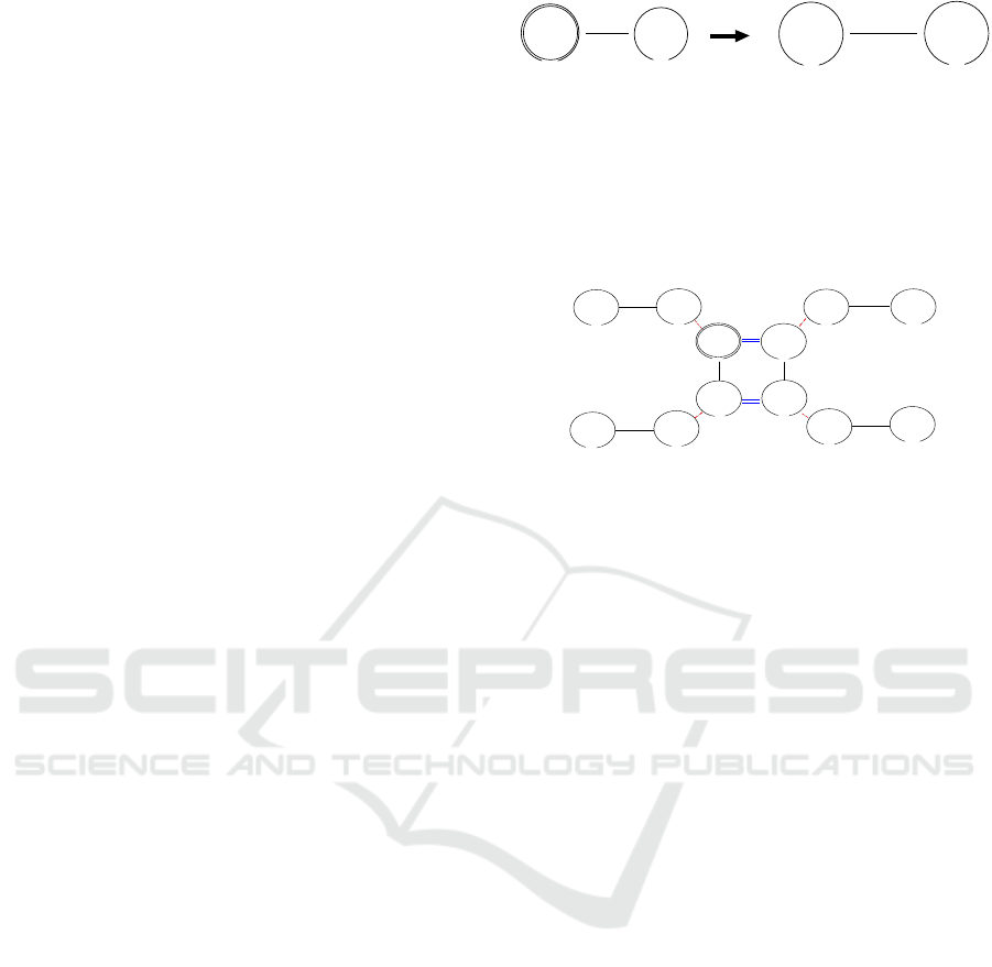
Figure 9 shows an example of a rule to implement
stretching spring. In the left part, an edge (that rep-
resents the spring) and their two extremities n0 and
n1 (where the force must be applied) were matched.
Here, we can see that a 0-link appears explicitly to
0
<
n0
>
n1
0
F_stretch:va...
n0
n1
3
2,
F_stretch:va...
<
>
3
2,
<
>
3
2,
<
>
3
2,
n0
<2,3>
0
Figure 9: Rule to compute a stretching springs forces.
bring out the two extremities of the edge, and the rest
of the edge orbit is expressed in the nodes. The right
part expresses that the force computed and stored in
the orbit h2, 3i of the vertex n0 and its opposite have
to be stored in the orbit h2, 3i of the vertex n1.
0
1
0
1
0 0
1
0
1
0
2
2
<>
nC
<>
<>
nE
n8
<>
nD
<>
<>
n2
<>
n5
<>
n13
<>
n10
<>
n8
n8
<>
n3
n8
<>
n4
n8
<>
n9
nF
<>
Figure 10: Matched pattern to compute angular springs
forces.
Another example that implements angular bend-
ing springs is represented in Figure 10. Here, we
present only the matched pattern (left part of the rule).
The edge which supports the spring constants can be
recognized by the four darts n3, n4, n8 and n9. The
sub-graph that allows one to find the vertices that
undergo the corresponding forces is also represented
(darts nc, nD, nE and nF). In the right part of the rule
(not presented), the angular spring’s forces are com-
puted for all concerned vertices and stored in the cor-
respond darts. The opposite of every force is applied
to the dart which is 0-linked (n2, n10, n5 and n13).
Figures 11 and 12 shows some results of our proto-
typing using mass/spring system and Figure 13, some
results using FEM.
Finally as described in the simulation loop, rules
are written to (1) collect all forces distributed in each
vertex sub-orbit, (2) find the acceleration, the new ve-
locity and the new position of each vertex. Symplec-
tic Euler has been used to integrate the equations of
motion. Combinations of rules can be written if more
complex schemes are used.
6 CONCLUSION AND FUTURE
WORK
The framework presented in this article aims at pro-
viding the existing physical models used in computer
graphics with a topological model. G-maps have been
chosen since they are more atomic and provide more
places to embed information than other models. All
mechanical data are stored directly in the G-map, and
GRAPP 2017 - International Conference on Computer Graphics Theory and Applications
226
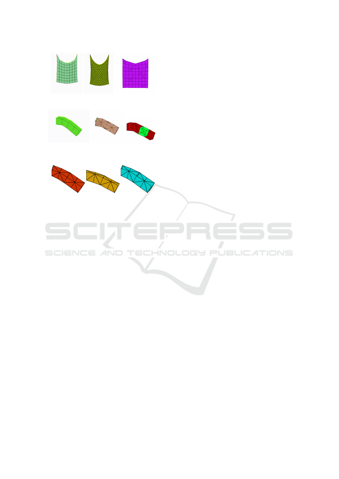
(a) Rectangular (b) Triangular (c) Mixed
Figure 11: Prototypes of mass/spring models in 2D.
(a) Hexahedral (b) Tetrahedral (c) Mixed
Figure 12: Prototyping of mass/spring models in 3D.
(a) FEM linear (b) Co-rotational (c) Mass/tensor
Figure 13: Prototyping of FEM models
the simulation uses neighboring relationships advan-
tageously.
Our model is completely general and generic.
First, it is independent on the dimension (2D,3D).
Second, it allows discrete or continuous interactions,
using the same general modeling process. Third,
based on sub-graph matching, our framework copes
with different types of elements and allows mixed
meshes.
Finally, a rule-based language has been used for
prototyping and building our simulation models. It
brings a graphical description of interactions and all
the necessary walks through the structure.
In future work, we want to test and enhance our
model with topological modifications, including mesh
adaptation or refinement. Last, considering that a
long-term evolution of JERBOA is to generate an op-
timized code implementing (in various languages in-
cluding C++) the rules that have been defined, we
hope to design a generator of physical models where
the user would only detail which forces the model
should undergo.
ACKNOWLEDGEMENTS
This work has been partially funded by the European
Erasmus Mundus - Al Idrisi II scholarship program.
It also received fundings from the MIRES federation.
Special thanks to Daniel Meneveaux for proofreading
and comments on this paper.
REFERENCES
Belhaouari, H., Arnould, A., LeGall, P., and Bellet, T.
(2014). Jerboa: A graph transformation library for
topology-based geometric modeling. In ICGT, pages
269–284.
Cotin, S., Delingette, H., and Ayache, N. (2000). A hybrid
elastic model allowing realtime cutting, deformation
and force feedback for surgery training and simula-
tion. Visual Computer, pages 437–452.
Damiand, G. and Lienhardt, P. (2014). Combinatorial
Maps: Efficient Data Structures for Computer Graph-
ics and Image Processing. A K Peter/CRC Press.
Etzmuss, O., Keckeisen, M., and Strasser, W. (2003). A fast
finite element solution for cloth modelling. In Pacific
Conference on Computer Graphics and Applications,
pages 244–251.
Fl
´
echon, E., Zara, F., Damiand, G., and Jaillet, F. (2013).
A generic topological framework for physical simula-
tion. In WSCG, pages 104–113.
Forest, C., Delingette, H., and Ayache, N. (2005). Remov-
ing tetrahedra from manifold tetrahedralisation: appli-
cation to real-time surgical simulation. Medical Image
Analysis, 9(2):113–122.
Golec, K., Coquet, M., Zara, F., and Damiand, G. (2015).
Improvement of a topological-physical model to man-
age different physical simulation. In WSCG, pages
25–34.
Grinspun, E., Hirani, A. N., Desbrun, M., and Schroder, P.
(2003). Discrete shells. In Symposium on Computer
Animation, pages 62–67.
Kjolstad, F., Kamil, S., Kelley, J. R., Levin, D. I. W., Shin-
jiro Sueda, D. C., Vouga, E., Kaufman, D. M., Kan-
war, G., Matusik, W., and Amarasinghe, S. P. (2016).
Simit: A language for physical simulations. ACM
Transactions on Graphics, 35.
Meseure, P., Darles, E., and Skapin, X. (2010). Topology
based physical simulation. In VRIPHYS, pages 1–10.
Nesme, M., Payan, Y., and Faure, F. (2005). Efficient,
physically plausible finite elements. In Eurographics,
pages 77–80.
O’Brien, J. F. and Hodgins, J. (1999). Graphical model-
ing and animation of brittle fracture. In SIGGRAPH,
pages 137–146.
Provot, X. (1995). Deformation constraints in a masss/pring
model to describe rigid cloth behaviour. In Graphics
Interface, pages 147–154.
Terzopoulos, D., Platt, J., Barr, A., and Fleischer, K. (1987).
Elastically deformable models. In SIGGRAPH, vol-
ume 21, pages 205–214.
A General Physical-topological Framework using Rule-based Language for Physical Simulation
227
