
Spatially Constrained Clustering to Define Geographical Rating
Territories
Shengkun Xie
1,3
, Zizhen Wang
2
and Anna Lawniczak
2
1
Department of Mathematical & Computational Sciences, University of Toronto Mississauga, Mississauga, Canada
2
Department of Mathematics and Statistics, University of Guelph, Guelph, Canada
3
Ted Rogers School of Management, Ryerson University, Toronto, Canada
shengkun.xie@utoronto.ca, shengkun.xie@ryerson.ca, zizhen@uoguelph.ca, alawnicz@uoguelph.ca
Keywords:
Spatially Constrained Clustering, Ratemaking, Geocoding, Gap Statistic, Business Data Analytic, Model
Selection.
Abstract:
In this work, spatially constrained clustering of insurance loss cost is studied. The study has demonstrated
that spatially constrained clustering is a promising technique for defining geographical rating territories using
auto insurance loss data as it is able to satisfy the contiguity constraint while implementing clustering. In
the presented work, to ensure statistically sound clustering, advanced statistical approaches, including average
silhouette statistic and Gap statistic, were used to determine the number of clusters. The proposed method
can also be applied to demographical data analysis and real estate data clustering due to the nature of spatial
constraint.
1 INTRODUCTION
Clustering analysis has been now widely used for
business analytic including automobile insurance
pricing as a machine learning tool (A.C. Yeo and
Brooks, 2001; Grize, 2015). It aims to partition
a set of multi-dimensional data to a limited size of
groups. It has also been used for territory analysis in
many states of USA where zip codes were treated as
an atomic geographical rating unit (Peck and Kuan,
1983). The aim of such analysis is to balance the
group homogeneity and the number of clusters de-
sired in order to ensure that insurance premium is fair
and credible. This is particularly important when in-
surance premium is regulated. The main focus of this
type of clustering is to determine an optimal parti-
tion of spatially constrained data into a set of groups,
based on some distance measures such as Euclidean
distance. The optimality is in the sense of being statis-
tically sound as well as being able to satisfy insurance
regulation. In clustering, the distance measures are
applied to each data dimension first and then the over-
all distance measure of each data point is compared to
each other to create different clusters or groups. How-
ever, how to handle the spatially constrained data in
clustering become a challenging task.
In determining a suitable insurance classification
of territory, average loss cost (or loss cost in short),
i.e. pure premium, is often used as one of the key vari-
ables to differentiate levels of loss for each designed
territory. Loss cost per geographical rating unit is cal-
culated by dividing the total loss per year (in terms of
dollars amount) within a given rating unit by the total
number of risk exposures, i.e., the number of vehicles
per year. The spatially constrained loss cost clustering
is not only of particular interest to insurance regula-
tors, who are mainly focusing on studying high level
statistics estimates, but also it is important for auto in-
surance companies, where accurate pricing based on
different territories are needed for the success of busi-
ness to avoid the adverse selection.
In this work, we aim for an optimal grouping strat-
egy for average loss costs at a Forward Sorting Area
(FSA) level. In Canada, a FSA consists of first three
letters of a postal code and it covers a much bigger
area than a single postal code does. This allows a
more reliable estimate of pure premium in a given
region of interest as it includes more risk exposures
(i.e., number of vehicles). Within insurance area, ge-
ographical information using postal codes has been
seriously considered for flood insurance pricing be-
cause the nature of insurance coverage is heavily de-
termined by geographical location of insureds. To our
best knowledge, the territory design using geo-coding
of FSAs has not appeared in the literature. This work
is considered as the first attempt on discussing this
82
Xie, S., Lawniczak, A. and Wang, Z.
Spatially Constrained Clustering to Define Geographical Rating Territories.
DOI: 10.5220/0006118100820088
In Proceedings of the 6th International Conference on Pattern Recognition Applications and Methods (ICPRAM 2017), pages 82-88
ISBN: 978-989-758-222-6
Copyright
c
2017 by SCITEPRESS – Science and Technology Publications, Lda. All rights reserved

topic.
In many countries including United States and
Canada, auto insurance rates are heavily regulated.
This implies that any rate-making methodology be-
ing used to analyze data must be both statistically
and actuarially sound. Ensuring statistical soundness,
it means that the approach being used must convey
meaningful statistical information and the obtained
results must be optimal in the statistical sense. From
the actuarial perspective, it requires that any proposed
rate-making methodology must take insurance regu-
lation and actuarial practice into consideration. For
example, loss cost must be at the similar level within
a given cluster and the total number of territories used
for insurance classification should be within a certain
range. Also, the number of exposures should be suf-
ficiently large to ensure that an estimate of statistics
from the given group is credible. Because of these,
it is critical to quantify the clustering effect and bal-
ance the results by taking both statistical soundness
and actuarial rate & class regulation requirements into
consideration.
The main contribution of this work is to propose
a spatially constrained clustering approach, which is
suitable for regional based business decision making
using analytical approach. The proposed method has
been applied to auto insurance pricing problem. Due
to the nature of this work, it is possible to apply this
method to other types of problems such as real estate
pattern analysis.
This paper is organized as follows. In Section
2, we discuss the proposed methods including rate-
making, clustering algorithms, and the choice of num-
ber of clusters. In Section 3, analysis of spatial loss
cost data and summary of main results are presented.
Finally, we conclude our findings and provide further
remarks in Section 4.
2 METHODS
In rate-making methodologiesfor auto insurance pric-
ing, territory design and analysis based on loss cost
of a geographical rating unit is one of the key aspects.
Loss cost is defined as a ratio of total loss to total
number of exposures. It is an average cost to cover
an exposure of risk for a given period (i.e., policy
term) and it is often called pure premium or theoreti-
cal premium. The need of territory design is to ensure
that the number of exposures in each territory is suf-
ficiently large so that the estimate of statistic within a
territory is credible. Also, the loss cost of basic rating
units within a territory must be at a similar level, i.e.
it must consider a suitable number of rating territo-
ries that satisfy contiguity constraint which ensure the
homogeneity and credibility for each territory. Often
large sizes of rating territories or a small total number
of rating territories easily satisfy the full credibility
requirement, but often not the homogeneity require-
ment. How to balance these two sides becomes the
major focus of this type of research. Also, each terri-
tory should contain only their neighbors, and cannot
include any rating units acrossing the boundaries be-
tween territories. This contiguity constraint inspires
us to consider a clustering with geocoding. Often we
refer this as a spatially constrained clustering.
2.1 Geocoding and Weighted Clustering
Auto insurance loss data contains residential infor-
mation of policy holders, i.e., postal codes, reported
claim information and others. The loss amount and
exposure of risk are then aggregated by postal codes
to derive loss cost. Often loss cost at postal code level
is less credible as it may not cover sufficient number
of reported claims for accurate analysis. Therefore,
in order to better reflect the nature of loss level, we
have to consider a rating unit that includes a larger
size of exposures, so that the loss cost estimate be-
comes more credible. In this work, we define FSA
as a basic geographical rating unit. This geographical
information is then coded into latitude and longitude.
The geocoding is then combined with other loss infor-
mation to become an input of a clustering algorithm.
We then consider an optimization problem that essen-
tially leads to a clustering algorithm, which can be
described as follows when taking K-mean as an ex-
ample.
Given a set of high dimensional observations
{X
1
, X
2
, ..., X
n
}, where each observation is a d-
dimensional real vector, i.e. X
i
∈ R
d
, a weighted K-
mean clustering aims to partition the n observations
into K sets (K ≤ n), S = {S
1
,S
2
,... ,S
K
}, so that it
minimizes the within-cluster sum of squares (WCSS):
argmin
S
K
∑
i=1
∑
X
j
∈S
i
kX
j
− µ
j
k
2
2
, (1)
where µ
i
is the mean point of the cluster S
i
. The
weighted sum of squares is defined as follows:
kX
j
− µ
j
k
2
2
=
d
∑
l=1
w
l
(x
jl
− µ
il
)
2
, (2)
where w
d
is used to specify the importanceness of
each dimension of data variable X
i
. In auto insurance
pricing, a typical focus on determining w
d
is to eval-
uate the importanceness of each pricing factor.
Often each dimension of data variable X
i
needs
to be scaled, i.e., a normalization procedure needs
Spatially Constrained Clustering to Define Geographical Rating Territories
83

to be applied before clustering. We assume that X
i
has been normalized. Specifically, in our case (i.e.,
when d = 3), µ
i
= (µ
i1
,µ
i2
,µ
i3
)
⊤
corresponds to mean
value of ith center of designed territory and X
j
=
(x
j1
,x
j2
,x
j3
)
⊤
is the vector consisting of the standard-
ized loss cost x
j1
, latitude x
j2
and longitude x
j3
of
the jth FSA, and w
d
is the weight applied to dth di-
mension of data variable. In this work, without loss
of generality, we take w
2
=w
3
=1 and we allow w
1
to
take different values. The idea is to define a relativ-
ity measure between loss cost and geographical loca-
tion as w
1
. When w
1
=1, the loss cost is deemed to be
as important as geographical information, while when
w
1
takes a value greater (less) than 1 the loss cost is
more (less) important than geographical information
in a clustering.
One can also use K-medoid clustering instead of
K-mean. The major difference between these two
approaches is estimate of the center of each cluster.
The K-mean clustering determines each cluster’s cen-
ter using the arithmetics means of each data charac-
teristic, while the K-medoid clustering uses the actu-
ally data points in a given cluster as the center. For
our clustering problem, it does not make any essen-
tial difference, which clustering method is selected,
as we aim for grouping only. Similarly, the hierar-
chical clustering, which seeks to build a hierarchy of
clusters, can also be considered.
2.2 Spatially Constrained Clustering
The K-mean or K-medoid clustering does not neces-
sarily lead to clustering results that satisfy the cluster
contiguity requirement. In this case, spatially con-
strained clustering is needed as all clusters are re-
quired to be spatially contiguous. We start from an
initial clustering. We assume that each cluster from
the initial clustering will contain only a few non-
contiguous points, and we just need to re-allocate
these points following an initial clustering. To re-
allocate these non-contiguous points, we first iden-
tify them, and then re-allocate them to the closest
(minimal-distance) point within a contiguous clus-
ter. In order to implement this allocation of non-
contiguous points, we propose an approach that is
based on Delaunay triangulation (Recchia, 2010;
Renka, 1996). In mathematics, a Delaunay triangu-
lation for a set P of points in a plane is a triangulation,
denoted by DT(P), such that no point in P is inside the
circumcircle of any triangle in DT(P). If a cluster P is
in DT(P) and DT(P) forms a convex hull (Preparata
and Hong, 1977), the clustering then satisfies the con-
tiguity constraint. In order to construct a DT, we pro-
pose the following procedure:
1. We first do K-mean clustering as an initial cluster-
ing.
2. Based on the obtained clustering results from the
previous step, we find all points that are entirely
surrounded by points from other clusters.
3. We then find the neighboring point at minimal dis-
tance to the point that has no neighbors in the
same cluster. We called the associated cluster as a
new cluster.
4. The points that have no neighbors are then reallo-
cated to new clusters.
It is possible that the reallocated points may still be
isolated, thus this entire routine should be iterated un-
til we find that no such isolated point exists. Note that
this implementation is purely based on algorithm we
develop and the boundary created for each cluster is
often not corresponding to the geographical bound-
ary of each basic rating unit. However, based on this
results, one should be able to further refine them to
ensure that the boundary of cluster is determined by
the boundary of FSAs.
2.3 Choice of the Number of Clusters
In data clustering, the number of clusters needs to be
determined first. In this work, the number of clus-
ters represents the number of territories. Finding opti-
mal number of clusters becomes especially challeng-
ing in high dimensional scenarios where visualiza-
tion of data is difficult. In order to be statistically
sound, several methods including average silhouette
(Rousseeuw, 1987) and gap statistic (R. Tibshirani
and Hastie, 2001) have been proposed for estimating
the number of clusters. The silhouette width of an
observation i is defined as
s(i) =
b(i) − a(i)
max{a(i),b(i)}
, (3)
where a(i) is the average distance between i and all
other observations in the same cluster and b(i) is the
minimum average distance between i to other obser-
vations in different clusters. Observations with large
s(i) (almost 1) are well-clustered, observations with
small s(i) (around 0) tend to lie between two clus-
ters and observations with negative s(i) are probably
placed in a wrong cluster.
Varying the total number of clusters from 1 to the
maximum total number of clusters K
max
, the observed
data can be clustered using any algorithm including
K-mean. Next average silhouette can be used to esti-
mate the number of components. For a given number
of clusters K, the overall average silhouette width for
ICPRAM 2017 - 6th International Conference on Pattern Recognition Applications and Methods
84
clustering can be calculated as
¯s =
n
∑
i=1
s(i)
n
. (4)
The number of clusters which gives the largest aver-
age silhouette width is used to estimate the optimal
number of clusters. Note that, the optimal number
of clusters may not be used eventually in practice,
given the fact that the real-world data is complex and
contains high level of variation. Often it is the case
that the optimal number of clusters provides a start-
ing point for clustering work and each cluster from
optimal clustering may be partitioned further in order
to improve the results.
Gap statistics, proposed by Tibshirani et al.
(2001), is another resampling-based approach for
determining the optimal number of clusters. This
method compares the observed distributionof the data
samples to a null reference distribution (such as uni-
form distribution). The number K of clusters is se-
lected such that K is the smallest value whose differ-
ence (i.e., gap) is statistically significant. The gap at
selected number K of clusters is defined as follows
Gap(K) = E
∗
N
[log(W
K
)] − log(W
K
) (5)
where W
K
is the within-cluster sum of squares and E
∗
N
is the expectation under a sample size of N from the
reference null distribution.
In order to compute the gap statistics,
E
∗
N
[log(W
K
)] needs to be determined first. This
is done by resampling from a given reference null
distribution and using A different reference distribu-
tions, as null distributions. Varying the total number
of clusters from 1 to K
max
, both the observed data and
the reference data are clustered. E
∗
N
[log(W
K
)] and the
standard deviation σ
K
are estimated as follows
E
∗
N
[log(W
K
)] =
1
A
A
∑
a=1
log(W
Ka
) (6)
and
σ
K
=
"
1
A
A
∑
a=1
{log(W
Ka
) − E
∗
N
[log(W
K
)]}
2
#
1/2
. (7)
The clustering result from the selected K clusters
is said to be statistically significantly different from
the null reference if
Gap(K) ≥ Gap(K + 1) − σ
K+1
p
1+ 1/A. (8)
The optimal K is the smallest value of K that achieves
this statistical significance. Similarly to the silhou-
ette statistic, due to the natural complexity and high
level of variation from real data as well as lack of
the certainty in selecting null distributions, the mean
and standard deviation computed by using A reference
distributions may lead to a significant bias. So in prac-
tice, the optimal number of clusters determined by (8)
only provides a starting point for further clustering
analysis of the data. In order to more systematically
select the suitable number of clusters, we propose a
refined approach based on (8). From (8), we derive
the following expression.
∆G(K) = Gap(K + 1) − Gap(K) ≤ σ
K+1
p
1+ 1/A.
(9)
Often A is large, therefore (10) suggest that an optimal
number is the smallest K which satisfies the corre-
sponding incremental Gap statistics which is less than
one standard deviation. This leads to the following
simplified version of (10)
∆G(K) = Gap(K + 1) − Gap(K) ≤ σ
K+1
. (10)
Furthermore, ∆G(K) fluctuates with K and the fluctu-
ation will distort the estimate of the optimal number
of clusters. Instead of looking for the smallest K that
satisfies the equation (11) based on the empirical pat-
tern, one can estimate the signal component of ∆G(K)
by imposing a power-law relationship.
−79.8 −79.7 −79.6 −79.5 −79.4 −79.3 −79.2
43.6 43.7 43.8 43.9
Longititude
Latitude
K−Medoid without Scaling
(a) K-Medoid
−79.8 −79.7 −79.6 −79.5 −79.4 −79.3 −79.2
43.6 43.7 43.8 43.9
Longititude
Latitude
K−Mean without Scaling
(b) K-Mean
−79.8 −79.7 −79.6 −79.5 −79.4 −79.3 −79.2
43.6 43.7 43.8 43.9
Longititude
Latitude
K−Medoid with Scaling
(c) K-Medoid
−79.8 −79.7 −79.6 −79.5 −79.4 −79.3 −79.2
43.6 43.7 43.8 43.9
Longititude
Latitude
K−Mean with Scaling
(d) K-Mean
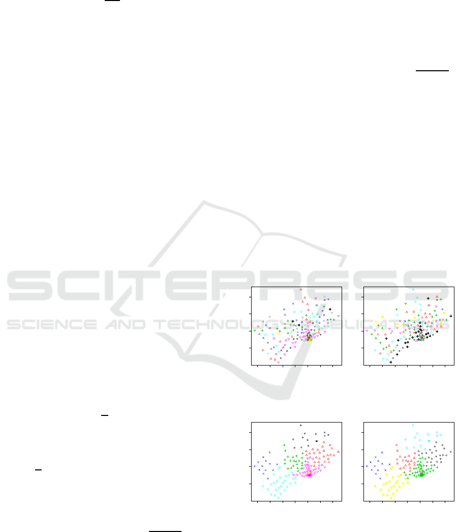
Figure 1: The clustering results using equal weight (i.e.,
w
1
=1) for the data with and without scaling. Each cluster
has the same color, and there are 10 clusters determined by
average silhouette method.
Spatially Constrained Clustering to Define Geographical Rating Territories
85
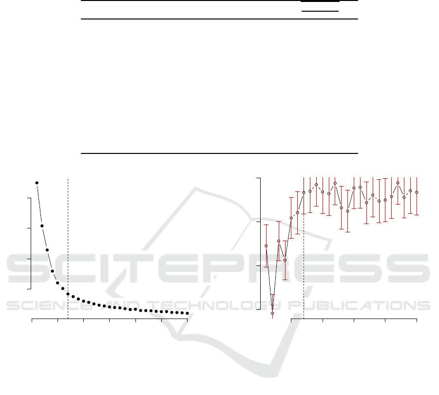
Table 1: The summary of model performance when the clustering results fitted to alinear model. An insurance claim frequency
of 2% and full credibility of 1082 claims are assumed for computing credibility of the minimum size of clusters, denoted by
min(E
i
).
w
1
K Std.Dev adjusted R
2
min(E
i
) min(
q
min(E
i
)∗2%
1082
,1)
0.5 4 672.8 0.5159 30,041 0.7452
0.6 4 672.8 0.5159 30,041 0.7452
0.7 3 867.6 0.1951 97,359 1
0.8 4 800.2 0.3152 54,092 0.9999
0.9 4 672.8 0.5159 30,041 0.7452
1.0 4 672.8 0.5159 30,041 0.7452
1.1 2 815.5 0.2889 159,966 1
1.2 2 815.5 0.2889 159,966 1
1.3 2 815.5 0.2889 159,966 1
1.4 2 815.5 0.2889 159,966 1
1.5 2 815.5 0.2889 159,966 1
1.6 7 408.3 0.8217 9,252 0.4135
0 5 10 15 20 25 30
100 200 300 400
Number of clusters K
Total within−clusters sum of squares
Figure 2: The selection of number of cluster based on el-
bow method using total within-clusters sum of squares. The
vertical dotted line is at K = 7, which is suggested by the
method.
3 RESULTS
In this section, we present the results of analysis using
a real data set from an auto insurance regulator. The
data consists of geographical information in terms of
FSAs, loss cost for each FSA, and exposures of risk
for each FSA. The number of exposures will be used
for credibility weighted and is not passed to a clus-
tering algorithm. Since the geo-coder takes only the
input of zip codes or postal codes, we first collect
all postal codes that are associated with each FSA.
Within each FSA, the postal codes are geo-coded. We
then use the geo-coding of postal codes within each
FSA to estimate the geo-coding of the given FSA sim-
5 10 15 20 25
0.70 0.75 0.80 0.85
Numbers of clusters K
Gap
k
Figure 3: The selection of number of clusters based on the
gap statistics. The vertical dotted line is at K = 7. The
vertical red bounded line indicates one standard deviation
region.
ply by taking the average of geo-coding along each
dimension. The obtained Latitude, Longitude and its
associated loss cost for each FSA becomes the input
of clustering algorithm.
Scaling of input data is an important procedure for
clustering. High data scale is not necessarily more
important than low scale of data. Here we demon-
strate the impact of scaling on clustering by compar-
ing results obtained from both with and without scal-
ing methods. In the case of without scaling of data
method, the clustering results shown in Figure 1 in
which K-mean and K-medoid methods are used, re-
spectively, suggest that the partitioning of input data
is not successful because the contiguity constraint of
clustering is not met. The interior of a cluster con-
ICPRAM 2017 - 6th International Conference on Pattern Recognition Applications and Methods
86
−79.8 −79.7 −79.6 −79.5 −79.4 −79.3 −79.2
43.6 43.7 43.8 43.9
Longititude
Latitude
1
2
3
4
5
6
7
8
9
10
11
12
13
14
15
16
17
18
19
20
21
22
Before
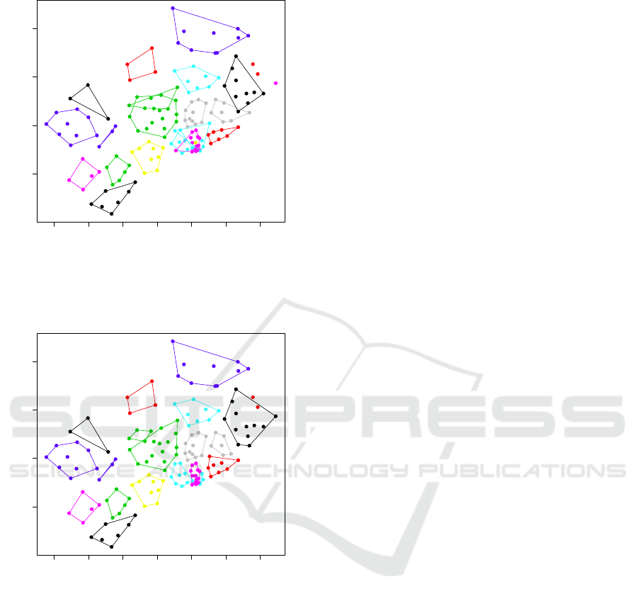
Figure 4: Convex hull plot of clusters obtained from the
K-mean clustering without re-allocation of isolated points.
−79.8 −79.7 −79.6 −79.5 −79.4 −79.3 −79.2
43.6 43.7 43.8 43.9
Longititude
Latitude
1
2
3
4
5
6
7
8
9
10
11
12
13
16
17
18
19
20
21
22
After
Figure 5: Convex hull plot of clusters obtained from the
K-mean clustering with re-allocation of isolated points.
tains elements from the other clusters. Even though
the sum of squares between the groups has explained
98.9% of the total sum of squares for a partition of
10 clusters, this partition of data does not satisfy the
insurance pricing regulation because of the contigu-
ity issue. When the input data is scaled, the clus-
tering results are more promising because they bet-
ter satisfy the contiguity constraint requirement. The
cost of having this better result is a lower proportion
of between groups variation, which is decreased from
98.9% to 81.5%. However, the contiguity constraint
is still not fully satisfied, because there exists some
points are isolated and within another cluster.
In order to produce the results of Figure 1, a
choice of the number of clusters was required. In this
paper, three methods including elbow method, aver-
age silhouette and gap statistic were used. For the
input data with scaling, 7 clusters were suggested by
both elbow method (qualitatively determined) and av-
erage silhouette method. The result of using elbow
method is shown in Figure 2. The choice of the num-
ber of clusters is based on the smallest K that is as-
sociated with insignificant decrease of within cluster
sum of squares. The selection of the number of clus-
ters using gap statistic is presented in Figure 3. When
applying either gap statistic and elbow method, the
optimal number of clusters should be determined with
care. For instance, gap statistic suggests the choice
of minimum K when the increment ∆G is larger than
σ
K+1
. When this choice is applied to our data, the
gap statistic suggests the number of clusters to be one,
which does not make sense as it suggest that no clus-
tering is required. This result is apparently due to the
heavy distortion caused by the underlying uncertainty
of the estimate of gap statistic and the standard devi-
ation. Therefore, a more suitable choice of K should
be made based on the overall pattern of gap statistic
with respect to K number of clusters. One should fo-
cus on the signal component of G(K) and select the
one that first approaches the stable state of gap statis-
tic. When this rule is applied, the similar number is
obtained to the ones obtained by the elbow method or
average silhouette method.
The clustering results are further analyzed by fit-
ting the data to ANOVA linear model. The ANOVA
model standard deviation and adjusted R
2
are ob-
tained from comparing the performance of model fit-
ting, in terms of predictive power (through adjusted
R
2
) and the model reliability (by looking at the model
standard deviation). From these results one can see
that the best performance is obtained when w
1
=1.6,
which means that the loss cost needs to be given more
weight. In this case, 7 clusters are suggested by the al-
gorithm in order to achieve the statistical soundness,
however this leads to a lower credibility. In calcu-
lating credibility, a 2% car insurance claim frequency
and full credibility of 1082 claims are assumed. This
further confirms that when the loss cost is given more
weight, the clustering is done mainly based on the
loss cost, and to satisfy the contiguity constraint, more
clusters may be needed.
To demonstrate the improvement of using spa-
tially constrained clustering that we proposed, we first
apply the K-mean clustering with w
1
=1 (i.e., being
equally important between the geophysical location
and the loss cost) using 22 clusters. The 22 clus-
ters were used by the regulator who owns the data
Spatially Constrained Clustering to Define Geographical Rating Territories
87

to come up with a design of territory for regulation
purpose. The result is shown in Figure 4. From this
result one can see that there are still many clusters,
such as 3, 13, 15, 21 and 18 (indicated within convex
hull), which do not satisfy the contiguity constraint
completely. Thus, we apply the proposed procedure
discussed in the methodology section to further refine
the results. From the output shown in Figure 5, all
the clusters form convex hull. Thus, the contiguity
constraint is satisfied.
4 DISCUSSIONS AND
CONCLUDING REMARKS
In this work, spatially constrained clustering of the in-
surance loss cost was studied. The FSAs represented
by their computed geocoding, and their associated in-
surance loss costs are the input of clustering algo-
rithms. The geocoding does not require a big extra ef-
fort as it can be easily obtained from some geo-coders
using Global Positioning System (GPS). In geocod-
ing of an FSA, each co-ordinate of centroid is deter-
mined by using the mean value of either latitude or
longitude value of the total postal codes within each
FSA. The geocoding and the loss cost values must be
standardized before using them in the clustering al-
gorithm. The standardization procedure is just a re-
location and re-scaling of each variable, i.e. loss cost,
latitude and longitude. The method of Delaunay tri-
angulation is used to ensure that the contiguity con-
straint is satisfied. In fact, the contiguity constraint
has many other applications in the earth and social
sciences and in image processing (Recchia, 2010). It
has been demonstrated that the spatially constrained
clustering is a promising approach for clustering in-
surance loss costs as it is able to satisfy the contigu-
ity constraint while implementing clustering. In the
presented work, to ensure clustering to be statistically
sound, advanced statistical approaches including av-
erage silhouette statistic and Gap statistic were used
to determine the number of clusters. The presented
work is based on data for all insurance coverage, it
may be interesting to see how the loss cost change
from one sub-coverage to another one. This needs to
be done by investigating sub-coverage data. Also, in
order to quantify the homogeneity of clustering, en-
tropy based method may be considered in future re-
search as it can measure how uniformity of the distri-
bution of loss cost is. The uniformity is what insur-
ance company expect to ensure that policyholders are
responsible for extract their cost.
ACKNOWLEDGEMENT
The Authors acknowledges support from NSERC
(Natural Sciences and Engineering Research Council
of Canada).
REFERENCES
A.C. Yeo, K.A. Smith, R. W. and Brooks, M. (2001). Clus-
tering technique for risk classification and prediction
of claim costs in the automobile insurance industry.
Intelligent Systems in Accounting, Finance and Man-
agement, 10:39 – 50.
Grize, Y. (2015). Applications of statistics in the field of
general insurance: An overview. International Statis-
tical Review, 83:135–159.
Peck, R. and Kuan, J. (1983). A statistical model of individ-
ual accident risk prediction using driver record, terri-
tory and other biographical factors. Accident Analysis
and Prevention, 15:371–393.
Preparata, F. and Hong, S. (1977). Convex hulls of finite
sets of points in two and three dimensions. Commun.
ACM, 20:87–93.
R. Tibshirani, G. W. and Hastie, T. (2001). Estimating the
number of clusters in a data set via the gap statistic.
Journal of the Royal Statistical Society: Series B (Sta-
tistical Methodology), 63:411–423.
Recchia, A. (2010). Contiguity-constrained hierarchical ag-
glomerative clustering using sas. Journal of Statistical
Software, 33:1–8.
Renka, R. (1996). Algorithm 772: Stripack: a
constrained two-dimensional delaunay triangulation
package. ACM Transactions on Mathematical Soft-
ware, 22:416–434.
Rousseeuw, P. (1987). Silhouettes: a graphical aid to the
interpretation and validation of cluster analysis. Com-
putational and Applied Mathematics, 20:53 – 65.
ICPRAM 2017 - 6th International Conference on Pattern Recognition Applications and Methods
88
