
Shape-based Trajectory Clustering
Telmo J. P. Pires and M
´
ario A. T. Figueiredo
Instituto de Telecomunicac¸
˜
oes and Instituto Superior T
´
ecnico, Universidade de Lisboa, Lisboa, Portugal
{telmopires, mario.figueiredo}@tecnico.ulisboa.pt
Keywords:
Unsupervised Learning, Directional Statistics, k-means, EM Algorithm, Nonnegative Matrix Factorization,
Trajectory Clustering.
Abstract:
Automatic trajectory classification has countless applications, ranging from the natural sciences, such as zo-
ology and meteorology, to urban planning, sports analysis, and surveillance, and has generated great research
interest. This paper proposes and evaluates three new methods for trajectory clustering, strictly based on the
trajectory shapes, thus invariant under changes in spatial position and scale (and, optionally, orientation). To
extract shape information, the trajectories are first uniformly resampled using splines, and then described by
the sequence of tangent angles at the resampled points. Dealing with angular data is challenging, namely due
to its periodic nature, which needs to be taken into account when designing any clustering technique. In this
context, we propose three methods: a variant of the k-means algorithm, based on a dissimilarity measure that
is adequate for angular data; a finite mixture of multivariate Von Mises distributions, which is fitted using
an EM algorithm; sparse nonnegative matrix factorization, using complex representation of the angular data.
Methods for the automatic selection of the number of clusters are also introduced. Finally, these techniques
are tested and compared on both real and synthetic data, demonstrating their viability.
1 INTRODUCTION
In recent years, an exponential growth in the amount
of available data for analysis has been experienced in
most fields of knowledge. These huge data quanti-
ties, far beyond the scope of manual analysis, have
stimulated a growing interest in automated methods.
Trajectory data is no exception, thanks to the grow-
ing number of tracking devices, including GPS re-
ceivers, RFID tags, tracking cameras, and even cell-
phone call traces (Becker et al., 2011). This has led to
a growing interest in automatic trajectory clustering,
as a means to perform activity recognition and clas-
sification. The study of traffic patterns, human mo-
bility, and even air pollution exposure of populations
(Demirbas et al., 2009); the detection of common be-
haviors in meteorological phenomena (Elsner, 2003);
animal movement analysis (Brillinger et al., 2004);
automated sports analysis; and automatic surveillance
are just a few of the applications of these techniques.
Besides being influenced by many factors not di-
rectly related to the phenomenon in study, such as sea-
sonality, in the case of hurricane tracks, trajectories
introduce many challenges by being represented by a
sequence of space-time data points:
1. Differences in the speed of tracked objects cause
misalignments in the trajectories, as illustrated in
Figure 1(a). Varying sampling rates have a similar
effect.
2. Similar trajectories may have a different number
of points, as illustrated in Figure 1(b).
3. In some applications, trajectories differing only in
a translation (and possibly orientation) should be
treated as being similar.
4. Besides being affected by noise, trajectories can
also have big, but sparse errors, called outliers.
(a) Objects moving at differ-
ent speeds, leading to mis-
aligned, but similar tracks.
(b) Similar tracks with a dif-
ferent number of points.
Figure 1: Some of the challenges faced with trajectory data.
In this paper, a novel approach is introduced for
Pires, T. and Figueiredo, M.
Shape-based Trajectory Clustering.
DOI: 10.5220/0006117400710081
In Proceedings of the 6th International Conference on Pattern Recognition Applications and Methods (ICPRAM 2017), pages 71-81
ISBN: 978-989-758-222-6
Copyright
c
2017 by SCITEPRESS – Science and Technology Publications, Lda. All rights reserved
71
clustering 2D trajectories, based exclusively on their
shapes. This means trajectories are clustered inde-
pendently of their location and of a global change of
scale. Optionally, it is also possible to have orienta-
tion invariance.
2 PREVIOUS WORKS
Other authors have studied the problem of trajectory
clustering. Their approaches can be divided into two
main groups: the distance metric approach and the
model based (generative) approach.
2.1 Distance Metric Approaches
These approaches aim to find (dis)similarity measures
between trajectories, and then cluster them based on
those measures. For example, the Euclidean distance
is used in (Fu et al., 2005) and (Hu et al., 2007),
which requires trajectories with the same number of
points and uniformly sampled, so a preprocessing step
is needed.
To avoid the need for uniformly sampled trajecto-
ries, methods that try to find an optimal alignment be-
tween time-varying sequences, such as dynamic time
warping (Pierobon et al., 2005) and longest common
subsequence (Vlachos et al., 2002) have been suc-
cessfully applied to trajectory clustering.
Another important method is TRACLUS (Lee
et al., 2007). This method allows sub-trajectory
clustering, instead of clustering the trajectories as a
whole, which may be useful in some applications.
This method works by partitioning trajectories in sub-
trajectories, and then performing density-based clus-
tering, using a specially defined metric.
2.2 Model-based Approaches
Model-based methods, on the other hand, attempt to
find a model capable of describing the whole dataset,
instead of directly comparing trajectories.
In (Gaffney and Smyth, 1999), trajectories are
represented as polynomial functions of time, and the
parameters of these functions are modeled as a finite
mixture. A similar approach is used in (Wei et al.,
2011), but trajectories are modeled using B-splines.
Another common approach to trajectory cluster-
ing models trajectories as vector fields. Some of these
works are (Ferreira et al., 2012), in which a variant of
k-means for vector fields was proposed, and (Nasci-
mento et al., 2013), where a mixture of vector fields
model allowing transitions between fields was pro-
posed.
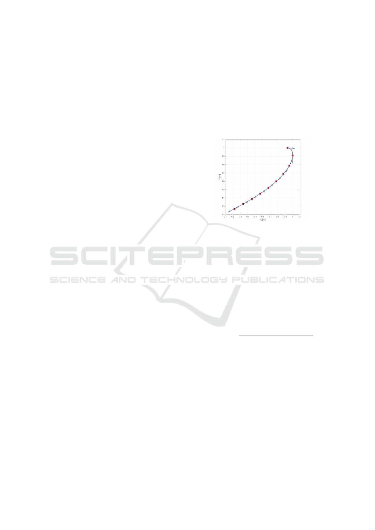
3 DATA PRE-PROCESSING
Trajectories are usually given as sequences of points,
so a pre-processing step is needed in order to capture
their shapes. In our case, shape is characterized as
a sequence of angles: the angles of the tangents to
the trajectory, sampled at uniformly spaced points, as
illustrated in Figure 2. As seen below, the sequence
of angles is invariant under changes in location and
scale of the trajectory.
Figure 2: Uniformly resampled trajectory and respective
tangents. Shape is characterized by the angles of the tan-
gent vectors w.r.t. the horizontal.
This pre-processing step solves the problem of tra-
jectories having different lengths and the problem of
misalignment, by assuring all trajectories are simi-
larly sampled. In this work, the resampling is per-
formed using cubic splines, fitted separately for both
the x and y coordinates. In order to fit splines, an
independent variable is needed, and it must be the
same for each coordinate. A natural choice is time,
but many datasets only have spatial information. In
these cases, the independent variable must be esti-
mated from data, using
τ
p+1
= τ
p
+
q
(x
(i)
p+1
− x
(i)
p
)
2
+ (y
(i)
p+1
− y
(i)
p
)
2
, (1)
with τ
1
= 0, where we assume that the speed is uni-
form.
To reduce the influence of noise, we use smooth-
ing splines, which are fitted by minimizing the cost
(De Boor, 2001)
p
m
∑
i=1
w
i
(x(τ
i
)− f (τ
i
))
2
+(1− p)
Z
(D
2
f (τ))
2
dτ, (2)
where p is a parameter that controls the trade-off be-
tween smoothness and accuracy, w
i
are weights we
set to 1, and D
2
f (τ) is the second derivative of func-
tion f . Many implementations of these algorithms are
readily available, such as the Curve Fitting toolbox in
MATLAB, which was used in this work.
ICPRAM 2017 - 6th International Conference on Pattern Recognition Applications and Methods
72

For a uniform resampling to d points, splines
should be evaluated at:
τ
i
= τ
1
+
τ
m
− τ
1
d − 1
(i − 1) , i = 1,.. . ,d,
where τ
1
and τ
m
are the τ’s calculated according to
Eq. (1).
The angles of the tangents are obtained by
ω
(i)
p
= atan2(D f
(i)
y
(τ
p
),D f
(i)
x
(τ
p
)) , ω
(i)
p
∈ [−π, π] ,
where atan2(·) is the 4-quadrant inverse tangent func-
tion and D f
(i)
y
(τ
p
) and D f
(i)
x
(τ
p
) refer to the first
derivatives of the fitted splines, evaluated at τ
p
. This
way, we get a d-dimensional vector ω
ω
ω
(i)
describing
the trajectory.
Besides being invariant to spatial translation and
scaling, another interesting property of this formula-
tion is that it allows trajectories to be invariant to ro-
tation with a small modification: by working with the
differences between consecutive angles, instead of the
angles themselves.
3.1 Choosing Parameters p and d
The pre-processing step requires two input parame-
ters: p and d. For choosing p, no systematic proce-
dure is available, and so we try several values until a
good one is found. The choice of d, on the other hand,
can be automated. This is done by finding the small-
est number of points that can accurately describe a
trajectory, called the characteristic points, which pro-
vides a lower bound for d, as the characteristic points
may not be equally spaced. In order to fully charac-
terize the trajectories, we use d approximately 5 times
the maximum number of characteristic points found
in the given dataset.
In (Lee et al., 2007), a method for finding the char-
acteristic points of a trajectory was proposed, which
uses the minimum description length (MDL) prin-
ciple. The idea is to loop though all the points in
a trajectory and to compute, MDL
par
(p
start
, p
curr
),
the MDL cost assuming p
start
and p
curr
are the only
characteristic points in the interval p
start
,. . ., p
curr
,
and MDL
nopar
(p
start index
, p
curr index
), the MDL cost
preserving the original trajectory. If MDL
par
≤
MDL
nopar
, then choosing p
curr
as a characteristic
point makes the MDL cost lower. This procedure is
shown in algorithm 1.
The MDL cost, or MDL length, of a given
partitioning consists of two components, L(H) and
L(D|H), given by
L(H) =
par
i
−1
∑
j=1
log
2
(length(p
c
j
p
c
j+1
)),
Algorithm 1: Approximate Trajectory Partitioning.
Input: A trajectory, as a sequence of points,
p
1
,. . ., p
m
Output: N
c
, the number of characteristic points
1 N
c
= 1 // Add the starting point
2 start index = 1 length = 1 while
start index + length ≤ m do
3 curr index = start index + length
cost
par
= MDL
par
(p
start index
, p
curr index
)
cost
nopar
=
MDL
nopar
(p
start index
, p
curr index
) if
cost
par
> cost
nopar
then
// Partition at the previous
point
4 N
c
= N
c
+ 1
start index = curr index − 1
length = 1
5 else
6 length = length + 1
7 end
8 end
9 N
c
= N
c
+ 1 // Add the ending point
L(D|H) =
par
i
−1
∑
j=1
c
j+1
−1
∑
k=c
j
h
log
2
(d
⊥
(p
c
j
p
c
j+1
, p
k
p
k+1
))
+ log
2
(d
θ
(p
c
j
p
c
j+1
, p
k
p
k+1
))
i
,
where par
i
is the number of characteristic points in
trajectory i, length(·) is the Euclidean length of a seg-
ment, p
a
p
b
is the segment defined by points p
a
and
p
b
and d
⊥
and d
θ
are the perpendicular and angular
distances, defined as:
d
⊥
(s
i
e
i
,s
j
e
j
) =
l
2
⊥1
+ l
2
⊥2
l
⊥1
+ l
⊥2
d
θ
(s
i
e
i
,s
j
e
j
) =
(
length(s
j
e
j
) × sin θ 0 ≤ θ < π/2
length(s
j
e
j
), π/2 ≤ θ ≤ π
where l
⊥1
and l
⊥2
are the distances illustrated in Fig-
ure 3.
Figure 3: Definition of distance functions from TRACLUS.
Image from (Lee et al., 2007).
To reduce the influence of noise in the procedure
above, we only apply it to estimate d after having
Shape-based Trajectory Clustering
73

smoothed the trajectories with the p given by the user
and using d twice the length of a trajectory, to assure
its shape is well captured.
From this point on, whenever we mention trajecto-
ries we mean the trajectories after pre-processing, i.e.,
the set {ω
ω
ω
(1)
,. . .,ω
ω
ω
(m)
}, where each trajectory ω
ω
ω
(i)
is
a sequence of angles (ω
(i)
1
,. . .,ω
(i)
d
).
4 K-MEANS
4.1 Introduction
The k-means algorithm is one of the most famous
clustering techniques (Jain, 2010), despite offering no
global optimality guarantees. Arguably, its popularity
is due to the fact that it is a very simple and fast ap-
proach to clustering.
Given a set of points and the number of de-
sired clusters, k-means stores a set of k centroids,
µ
µ
µ
1
,. . .,µ
µ
µ
k
, and alternates between two steps: assign-
ment and centroid update.
1. Assignment step: set c
(i)
:= arg min
j
kx
x
x
(i)
− µ
µ
µ
j
k
2
for all i, where c
(i)
= j if the ith input sample be-
longs to cluster j. In other words, assign each
sample to the closest centroid. Possible ties are
broken by some arbitrary rule.
2. Centroid update step: set µ
µ
µ
j
:=
∑
m
i=1
1{c
(i)
= j}x
x
x
(i)
∑
m
i=1
1{c
(i)
= j}
for
all j, where 1{c
(i)
= j} is an indicator function,
taking the value 1 if c
(i)
= j and 0 otherwise, that
is, move each centroid to the mean of the points
assigned to it.
Originally, k-means was developed to work with
Euclidean distances, although many other versions
have been proposed in the literature. In our case, we
need to adapt it to handle the sequences of angles that
describe each trajectory.
4.2 Measuring Distances
A classical measure of the distance between two an-
gles is the length of the chord between them, as illus-
trated in Figure 4. It can be shown that, if the dif-
ference between two angles is ∆ω, the length of the
corresponding chord (red line in Fig. 4) is given by
2sin
∆ω
2
. Since sin is an odd function, it returns a
negative length if the angular difference is negative.
This is unintended, so we take the squares,
Figure 4: Relationship between angular difference and
chord (in red) in a unit circle.
2sin
∆ω
2
2
= 2 (1 − cos ∆ω) ∝ 1 − cos ∆ω,
where the constant “2” is irrelevant and dropped,
since this function will only be used to compare dis-
tances. Thus, the final metric is 1 − cos ∆ω. The
extension of this expression to d-dimensional data is
trivial:
D
2
(ω
ω
ω
(1)
,ω
ω
ω
(2)
) =
d
∑
p=1
1 − cos(ω
(1)
p
− ω
(2)
p
)
, (3)
where the ω
ω
ω
(i)
’s are angular vectors and ω
(i)
p
is the
pth component of vector i. The notation D
2
is used to
indicate this metric is a squared value (of the chord).
4.3 Updating the Centroids
The arithmetic mean cannot be used for updating the
coordinates of a centroid, as it does not work well
with circular data. In this work, we define the mean
of a sequence of angles {ω
(1)
,. . .,ω
(m)
} as:
¯
ω = atan2
1
m
∑
m
i=1
sinω
(i)
1
m
∑
m
i=1
cosω
(i)
!
(4)
The extension of this result to vectorial data is
straightforward: the mean of an angular vector is the
angular mean of each of its coordinates.
4.4 Algorithm Description
For the algorithm to be completely described, initial-
ization and stopping criteria must be specified. Re-
garding initialization, k-means++ (Arthur and Vassil-
vitskii, 2007) is used, but using Eq. (3) instead of
the Euclidean distance. The termination condition is
when the assignments no longer change between con-
secutive iterations.
ICPRAM 2017 - 6th International Conference on Pattern Recognition Applications and Methods
74

Algorithm 2: circular k − means algorithm.
Input: Data set, {ω
ω
ω
(1)
,. . .,ω
ω
ω
(m)
}, and number
of clusters, k
Output: Cluster centroids, µ
µ
µ
1
,. . .,µ
µ
µ
k
, and
cluster assignments, c
(1)
,. . .,c
(m)
1 Initialize k cluster centroids: µ
µ
µ
1
,. . .,µ
µ
µ
k
2 repeat
3 foreach i do
4 Set c
(i)
:= arg min
j
D(ω
ω
ω
(i)
,µ
µ
µ
j
)
// Assign centroids to samples
5 end
6 foreach j do
7 Set µ
p
j
= atan2
∑
m
i=1
1{c
(i)
= j}sin ω
(i)
p
∑
m
i=1
1{c
(i)
= j}cos ω
(i)
p
for p = 1,... ,d // Update each
coordinate of the centroids
8 end
9 until convergence
4.5 Model Selection
In real-world situations, the number of clusters, k, is
not given, and it is necessary to estimate it. One com-
mon choice used in conjunction with k-means is the
so-called elbow method. This method involves com-
puting a distortion function for several values of k and
finding an elbow, that is, a point after which the rate of
decrease is significantly smaller. The distortion func-
tion is just the sum of the distances of each data sam-
ple to the respective centroid. For circular k-means,
this is given by
J(ω
ω
ω
(1)
,. . .,ω
ω
ω
(m)
,c
(1)
,. . .,c
(m)
,µ
µ
µ
1
,. . .,µ
µ
µ
k
)
=
m
∑
i=1
d
∑
p=1
1 − cos(ω
(i)
p
− µ
p
c
(i)
)
.
5 FINITE MIXTURE MODELS
Given a set of d-dimensional trajectories,
{ω
ω
ω
(1)
,. . .,ω
ω
ω
(m)
}, which is to be partitioned into
k clusters, we can model this set as i.i.d. samples of a
finite mixture,
p(ω
ω
ω
(i)
|θ
θ
θ) =
k
∑
j=1
α
j
p(ω
ω
ω
(i)
|z
(i)
= j,θ
θ
θ),
where the z
(i)
’s are latent variables, with z
(i)
= j
meaning the ith trajectory belongs to cluster j. Each
parameter α
j
= p(z
(i)
= j) is the mixing probability,
and θ
θ
θ a set of parameters characterizing the distribu-
tions. The likelihood function of the given set of tra-
jectories can be written as
p(ω
ω
ω
(1)
,. . .,ω
ω
ω
(m)
|α
α
α,θ
θ
θ) =
m
∏
i=1
p(ω
ω
ω
(i)
|α
α
α,θ
θ
θ)
=
m
∏
i=1
k
∑
j=1
α
j
p(ω
ω
ω
(i)
|z
(i)
= j,θ
θ
θ). (5)
A popular distribution for modeling circular data
is the Von Mises distribution, making it a natu-
ral choice for our mixture model. This way, the
p(ω
ω
ω
(i)
|z
(i)
= j,θ
θ
θ) are Von Mises pdf’s. The pdf of
a multivariate Von Mises is (Mardia et al., 2008)
p(ω
ω
ω;µ
µ
µ,κ
κ
κ,Λ
Λ
Λ) = T (κ
κ
κ,Λ
Λ
Λ)
−1
exp
κ
κ
κ
T
c(ω
ω
ω,µ
µ
µ)
+
1
2
s(ω
ω
ω,µ
µ
µ)
T
Λ
Λ
Λ s(ω
ω
ω,µ
µ
µ)
, (6)
where
c(ω
ω
ω,µ
µ
µ)
T
= [cos(ω
1
− µ
1
), ... , cos(ω
d
− µ
d
)],
s(ω
ω
ω,µ
µ
µ)
T
= [sin(ω
1
− µ
1
), ... , sin(ω
d
− µ
d
)],
and T (κ
κ
κ,Λ
Λ
Λ)
−1
is a normalizing constant, which is un-
known in explicit form for d > 2. Parameters µ
µ
µ and
κ
κ
κ are the d-dimensional mean and concentration of
the distribution; Λ
Λ
Λ is a d × d symmetric matrix (with
zeros in the diagonal), where entry Λ
i j
measures the
dependence between ω
i
and ω
j
. Matrix Λ
Λ
Λ can be seen
as the analogous to the covariance matrix in a Gaus-
sian distribution.
The usual choice for obtaining maximum like-
lihood (ML) or maximum a posteriori (MAP) esti-
mates of the mixture parameters is the EM algorithm
(Dempster et al., 1977), which is an iterative proce-
dure with two steps:
• E-step: Set w
(i)
j
= p(z
(i)
= j|ω
ω
ω
(i)
;α
α
α,M
M
M,K
K
K, L
L
L),
where M
M
M, K
K
K, and L
L
L are used in place of
{µ
µ
µ
1
,. . .,µ
µ
µ
k
}, {κ
κ
κ
1
,. . .,κ
κ
κ
k
}, and {Λ
Λ
Λ
1
,. . .,Λ
Λ
Λ
k
}, re-
spectively.
Using Bayes’ Theorem, the E-step reduces to
computing, for every i and j,
w
(i)
j
=
α
j
p(ω
ω
ω
(i)
|z
(i)
= j; µ
µ
µ
j
,κ
κ
κ
j
,Λ
Λ
Λ
j
)
∑
k
l=1
α
l
p(ω
ω
ω
(i)
|z
(i)
= l; µ
µ
µ
l
,κ
κ
κ
l
,Λ
Λ
Λ
l
)
, (7)
where p(ω
ω
ω
(i)
|z
(i)
= j;µ
µ
µ
j
,κ
κ
κ
j
,Λ
Λ
Λ
j
) is a multivariate
Von Mises pdf.
• M-step: this step requires maximizing the follow-
ing function, with respect to the parameters of the
model:
∑
m
i=1
∑
k
j=1
w
(i)
j
ln
p(ω
ω
ω
(i)
|z
(i)
= j;µ
µ
µ
j
,κ
κ
κ
j
,Λ
Λ
Λ
j
)p(z
(i)
= j;α
α
α)
w
(i)
j
Shape-based Trajectory Clustering
75

The multivariate Von Mises pdf depends on
T (κ
κ
κ
j
,Λ
Λ
Λ
j
), an unknown constant, which presents
a challenge for ML or MAP estimation. To avoid
having to use special numeric procedures, we as-
sume that the components of the ω
ω
ω
(i)
vector are
independent of the others, which makes the mul-
tivariate Von Mises distribution equivalent to the
product of d (the number of features) univariate
Von Mises distributions:
p(ω
ω
ω
(i)
|z
(i)
= j; µ
µ
µ
j
,κ
κ
κ
j
,Λ
Λ
Λ
j
) =
d
∏
p=1
e
κ
p
j
cos(ω
(i)
p
−µ
p
j
)
2πI
0
(κ
p
j
)
,
(8)
where µ
p
j
, κ
p
j
, and ω
(i)
p
refer to the pth component
of vectors µ
µ
µ
j
, κ
κ
κ
j
and ω
ω
ω
(i)
, respectively, and I
0
is
the modified Bessel function of first kind and or-
der 0.
Using ML estimation, the update equations for µ
q
l
(the qth component of µ
µ
µ
l
), α
l
and κ
q
l
are as fol-
lows:
µ
q
l
= atan2
∑
m
i=1
w
(i)
l
sinω
(i)
q
∑
m
i=1
w
(i)
l
cosω
(i)
q
!
, (9)
α
l
=
1
m
m
∑
i=1
w
(i)
l
, (10)
κ
q
l
= A
−1
1
∑
m
i=1
w
(i)
l
cos(ω
(i)
q
− µ
q
l
)
∑
m
i=1
w
(i)
l
!
, (11)
where A
1
(·) =
I
1
(·)
I
0
(·)
, with I
1
and I
0
denoting the
modified Bessel functions of the first kind and or-
ders 1 and 0, respectively.
In some cases, it is of interest to restrict κ
κ
κ
l
, in
order to avoid overfitting small datasets. We refer
to this variant as a constrained Von Mises mixture
(VMM), as opposed to the unconstrained (previous)
case. To constrain the concentration parameter, the
components of the κ
κ
κ
l
are forced to be the same, i.e.,
κ
1
l
= κ
2
l
= . . . = κ
d
l
= κ
l
, so (11) is replaced by
κ
l
= A
−1
1
1
d
d
∑
p=1
∑
m
i=1
w
(i)
l
cos(ω
(i)
p
− µ
p
l
)
∑
m
i=1
w
(i)
l
!
. (12)
5.1 Prior on the Concentration
Parameter
Due to the asymptotic behavior of the A
−1
1
function,
the estimation of the concentration parameter is prone
to numerical problems. One way to deal with this is
to introduce a prior, limiting its range of possible val-
ues. In this work, the conjugate prior of the Von Mises
distribution is used (Fink, 1997),
p(κ;c, R
0
) =
(
1
K
e
κR
0
I
0
(κ)
c
, κ > 0
0 , otherwise,
(13)
where K =
R
∞
0
e
κR
0
I
0
(κ)
c
is a normalizing constant, and
c > 0 and R
0
≤ c are parameters that control the shape
of the prior. Using this prior, the update rule for κ
q
l
is:
κ
q
l
= A
−1
1
1
1+c
∑
m
i=1
w
(i)
l
cos(ω
(i)
q
−µ
q
l
)
∑
m
i=1
w
(i)
l
+ R
0
.
(14)
When constraining κ
κ
κ
l
, a similar expression is ob-
tained, but whose argument is averaged over the d di-
mensions.
5.2 Algorithm Description
Algorithm 3: Mixture of Von Mises for trajectory
clustering algorithm.
Input: {ω
ω
ω
(1)
,. . .,ω
ω
ω
(m)
} and the number of
clusters, k
Output: {µ
µ
µ
1
,. . .,µ
µ
µ
k
}, {κ
κ
κ
1
,. . .,κ
κ
κ
k
} and α
α
α
1 Initialize α
α
α, {µ
µ
µ
1
,. . .,µ
µ
µ
k
}, {κ
κ
κ
1
,. . .,κ
κ
κ
k
}
2 repeat
// E-step
3 foreach i, j do
4 Set w
(i)
j
:=
α
j
p(ω
ω
ω
(i)
|z
(i)
= j;µ
µ
µ
j
,κ
κ
κ
j
)
∑
k
j=1
α
j
p(ω
ω
ω
(i)
|z
(i)
=l;µ
µ
µ
j
,κ
κ
κ
j
)
5 end
// M-step
6 Update α
j
with Eq. (10) for j = 1..., k
7 Update µ
p
j
with Eq. (9) for j = 1..., k and
p = 1,.. . ,d
8 Update κ
p
j
with Eq. (11), (12), or (14) for
j = 1 ..., k and p = 1,. ..,d
9 until convergence condition is satisfied
// Compute cluster assignments
10 foreach i = 1,. ..,m do
11 c
(i)
= arg max
j=1,...,k
w
(i)
j
12 end
To completely described the algorithm, an ini-
tialization procedure and a termination condition are
needed. Regarding initialization, we set α
j
=
1
/
k
,∀ j,
that is, we assume all clusters are equally likely; κ
κ
κ
j
is
initialized with the global κ over all dimensions and
all samples; the centroids are initialized with the re-
sults of running k-means with k-means++ initializa-
tion. Regarding termination, the algorithms are exe-
cuted until the change in log-likelihood is less than a
fraction ε = 10
−4
of its current value.
ICPRAM 2017 - 6th International Conference on Pattern Recognition Applications and Methods
76

5.3 Model Selection
One advantage of using probabilistic methods is the
ability to use formal approaches for model selection,
such as the MDL principle (Lee, 2001), (Rissanen,
1978).
The MDL cost has two components: the length of
the model, L(H), and the length of data encoded with
the model, L(D|H). In our case, the MDL cost can be
shown to be
MDL
cost
=
−
m
∑
i=1
ln
k
∑
j=1
α
j
p(ω
ω
ω
(i)
|z
(i)
= j,µ
µ
µ
j
,κ
κ
κ
j
) +
c
2
lnm,
where c is the number of parameters of the model.
For unconstrained VMM’s, c = k × (2d + 1); for con-
strained, c = k × (d + 2).
For selecting the number of clusters, several val-
ues are tried, and the one minimizing the MDL cost
is chosen. To avoid local optima, EM is run several
times for each k, and only the highest likelihood solu-
tion is considered (Lee, 2001).
6 MATRIX FACTORIZATION
Nonnegative matrix factorization (NMF) is a special
type of matrix factorization where a nonnegative data
matrix, V , is decomposed as the product of two low-
rank matrices, W and H, also nonnegative (Lee and
Seung, 1999). One of the many reasons for the re-
cent interest NMF has received is its close relation-
ship with k-means. In fact, it has been shown that it
is equivalent to k-means, with appropriate constraints.
Since we are sometimes interested in factorizing ma-
trices with negative entries, variants such as semi-
NMF have been proposed (Caner T
¨
urkmen, 2015).
Unfortunately, the constraints that make NMF
equivalent to k-means lead to an intractable problem,
thus they must be relaxed. One way to do this is
by using sparse semi-NMF (SSNMF) (Li and Ngom,
2013), which solves the following optimization prob-
lem:
min
W,H≥0
"
kV −W Hk
2
F
+ ηkW k
2
F
+ β
m
∑
i=1
|h
h
h
i
|
2
#
, (15)
where |h
h
h
i
| is the `
1
-norm of the ith column of H, while
η and β are tuning parameters: η > 0 controls the size
of the elements of W, while β > 0 controls the trade-
off between sparseness and accuracy of the approxi-
mation.
6.1 Application to Circular Data
Unfortunately, the standard factorization techniques
do not directly work with circular data. One way
to deal with this is to convert the angles to unit vec-
tors, which do not have the problems of circular data.
This can be done by stacking the set of trajectories,
{ω
ω
ω
(1)
,. . .,ω
ω
ω
(m)
}, as columns of the Ω
Ω
Ω matrix, and use
the duality between 2D vectors and complex numbers.
This way, we can define matrix V as:
V = e
jΩ
Ω
Ω
=
| | |
e
jω
ω
ω
(1)
e
jω
ω
ω
(2)
·· · e
jω
ω
ω
(m)
| | |
,
where j is the imaginary unit and e
jω
ω
ω
(i)
is the complex
vector:
e
jω
ω
ω
(i)
=
e
jω
(i)
1
,. . .,e
jω
(i)
d
T
,
where ω
(i)
p
is the pth entry of trajectory ω
ω
ω
(i)
. In this
work we use the exponential of a matrix as the expo-
nential of its entries. It can be shown that factorizing
this matrix is approximately equivalent to minimizing
the squares of the chords corresponding to the differ-
ences between angles.
Using this matrix, we may use SSNMF for clus-
tering. One last step can be applied to avoid work-
ing with complex valued matrices: since the real and
imaginary parts of matrix V are treated independently,
one can get the same results by factorizing V
0
instead,
where
V
0
=
ℜ{e
jΩ
Ω
Ω
}
ℑ{e
jΩ
Ω
Ω
}
. (16)
The W matrix will change by a similar transformation.
Since we are only interested in the angles, and not the
vectors themselves, the matrix of the shape centroids
is
W = arg
W
0
1
+ jW
0
2
, (17)
where W
0
1
and W
0
2
are, respectively, the top and bottom
halves of the W
0
matrix obtained by factorizing V
0
.
Function arg(·) returns the argument of each entry of
the input matrix. In this work, “The NMF MATLAB
Toolbox” was used (Li and Ngom, 2013).
6.2 Algorithm Description
The complete clustering algorithm using SSNMF is
described in Algorithm 4.
The η parameter is set to 0 in our tests, as there is
no interest in constraining the W matrix. For β, the
default value is 0.1.
Shape-based Trajectory Clustering
77

Algorithm 4: Sparse NMF applied to clustering of tra-
jectories.
Input: Set of trajectories, {ω
ω
ω
(1)
,. . .,ω
ω
ω
(m)
},
number of desired clusters, k and η and
β parameters
Output: Clustering assignments, c
(i)
’s, and, if
needed, centroid matrix, W
1 Compute V
0
matrix from Eq. (16).
2 Using “The NMF MATLAB Toolbox”, find W
0
and H minimizing Eq. (15).
3 Compute W from Eq. (17). // Compute
cluster assignments
4 foreach i = 1,. ..,m do
5 c
(i)
= arg max
j=1,...,k
H
ji
6 end
6.3 Model Selection
The MDL principle can not be directly applied to SS-
NMF, but other methods can be used. The elbow
method works as for k-means, but uses a different cost
function: J(V
0
,W
0
,H) = kV
0
−W
0
Hk
2
F
. The so-called
consistency method works as follows (Kim and Park,
2008):
1. For each k, compute the consistency matrix:
C
k
(i, j) = 1 ⇐⇒ i and j are in the same cluster
2. Repeat the previous step multiple times, and com-
pute the mean consistency matrix.
3. Finally, compute the consistency of each cluster-
ing using:
ρ
k
=
1
n
2
m
∑
i=1
m
∑
j=1
4
ˆ
C
k
(i, j) −
1
2
2
, 0 ≤ ρ
k
≤ 1,
and choose k where ρ
k
drops.
The reasoning behind this choice for k is that, for
the right k, SSNMF should be consistent, but not for
higher k’s. For smaller ones, it may or may not be so.
7 RESULTS
In this section, k-means, unconstrained and con-
strained VMM’s, and SSNMF are tested and com-
pared, on both synthetic and real datasets.
7.1 Synthetic Datasets
The performance of the proposed algorithms is ana-
lyzed using the following two datasets:
• The roundabout dataset (Figure 5) models a
roundabout where vehicles enter at the bottom and
circulate counterclockwise. There are 4 possible
exits, and each of these 4 clusters is composed of
20 noiseless trajectories. The radius and the cen-
ter of the roundabout were randomly generated for
each trajectory, making their shapes a little differ-
ent.
Figure 5: Roundabout synthetic dataset and its 4 clusters.
• The circles dataset (Figure 6) shows 100 circular
trajectories, in 4 equal size clusters. The top two
clusters correspond to objects circulating counter-
clockwise, while the bottom two, to objects circu-
lating clockwise. The radius and center of each
trajectory change between samples, and each tra-
jectory starts at a random orientation in the inter-
val [0,2π[. To ignore the changes in orientation,
we cluster the differences between angles of the
tangents, instead of the angles themselves. This
way, there are two distinguishable clusters in the
dataset, composed by the top and bottom circles.
Figure 6: Circles dataset and its 2 clusters. The two top
circles rotate counterclockwise, while the bottom two rotate
clockwise.
• The Noisy dataset (Figure 7(a)) was designed for
testing the effect of noise on the performance
of the algorithms. This dataset has 4 clusters,
with 50 trajectories each, and is corrupted by zero
mean Gaussian noise, with a standard deviation of
1.5 m.
ICPRAM 2017 - 6th International Conference on Pattern Recognition Applications and Methods
78

• The Concentration dataset (Figure 7(b)) was cre-
ated to illustrate the advantages of probabilis-
tic modeling (VMM’s) over the other techniques.
This dataset contains 100 trajectories, equally dis-
tributed between the two clusters, and was gener-
ated by the same mean trajectory, but with differ-
ent variances (standard deviations of 0.5 m and 2
m).
(a) Noisy Tracks synthetic
dataset, with 4 clusters.
(b) Concentration dataset
and its 2 clusters.
Figure 7: Noisy datasets.
For the noiseless and Concentration datasets, no
smoothing was used. For the Noisy dataset, several
possible values for p were tested. In the noiseless
datasets, 50 features were used, and 30 in the other
two. Each of the 4 clustering algorithms was run on
these datasets and given the right number of clusters.
This was repeated 1000 times, and the percentage of
trials the correct clustering was found is shown in Ta-
ble 1.
Table 1: Percentage of times the optimal assignment was
achieved out of 1000 trials in the synthetic datasets. The ‘*’
indicate numerical issues.
Dataset k-means unconstrained VMM constrained VMM SSNMF
Roundabout 96.7% 96.7% 96.7% 100.0%
Circles 100.0% 100.0%* 100.0%* 100.0%
Noisy (p = 1) 58.1% 58.4% 58.4% 42.6%
Noisy (p = 0.5) 58.8% 59.0% 59.0% 64.3%
Noisy (p = 0.1) 65.4% 65.4% 65.4% 83.6%
Noisy (p = 0.01) 82.4% 82.4% 82.4% 92.4%
Noisy (p = 1e − 5) 99.1% 99.1% 99.1% 35.7%
Noisy (p = 0) 99.7% 99.7% 99.7% 34.6%
Concentration 0.0% 68.9% 79.4% 0.0%
In both noiseless datasets, the true clusterings
were found most of the time. There were some nu-
merical issues with the circles dataset, as the trajec-
tories are too similar. To avoid this, a prior with
c = −R
0
= 5e − 5 was introduced and used in this
and all the following tests. In the Noisy dataset, it
was observed that below a certain level of smooth-
ing, all algorithms performed better with the decrease
in p. Stronger smoothing led to poorer results for
SSNMF, but better for the other methods. It is impor-
tant to note, however, that shape information is lost
with too much smoothing, so it is not advised. Over-
all, the best results were obtained for p = 0.01. In the
Concentration dataset, only the VMM’s were able to
find the right clusters, as expected. It is interesting
to note that the constrained version outperformed the
unconstrained one, probably due to the latter having
too many degrees of freedom for the available dataset.
7.2 Influence of β on SSNMF Results
In the previous tests, the β parameter of SSNMF was
set to 0.1. To determine its effect on the results,
a parametric study was conducted, using the Noisy
dataset. With p = 0.01, β was varied, and the tests
were repeated 100 times. Table 2 summarizes the re-
sults. For β ∈ [0.1,0.5], performance is approximately
constant, thus justifying the choice of β used. Low
and high β’s give poorer results.
Table 2: Percentage of times the optimal assignment was
achieved out of 100 trials for various values for β.
β 0 10
−3
0.01 0.1 0.2 0.5 1 2 5 10
Results 1% 32% 92% 94% 92% 91% 82% 63% 61% 63%
7.3 Model Selection on the Synthetic
Datasets
In the previous tests, the algorithms were given the
correct number of clusters. Since this is not the case
in real problems, we now evaluate the model selection
criteria. For this, k was varied in the range 1, . .., 10
and the tests were repeated 20 times for each k, to
avoid local optima, for each dataset and algorithm.
A parametric study of the influence of p on model
selection was also performed. Results are shown in
tables 3 and 4.
In the noiseless datasets, the elbow method (us-
ing k-means and SSNMF) found the right number of
clusters. MDL minimization using an unconstrained
VMM also found the right k in these cases and in
the Concentration dataset. In the noisy dataset, only
MDL minimization using an unconstrained VMM
found the true k, except for very small p’s. This
is because too much smoothing makes local patterns
emerge, and also causes higher likelihoods. The other
two criteria, MDL minimization using constrained
VMM’s and consistency performed poorly. The for-
mer performed poorly because the VMM uses very
few parameters, and so too complex models are not
penalized enough. The latter, on the other hand, per-
formed badly because SSNMF was consistent even
for values of k higher than the true one.
Shape-based Trajectory Clustering
79
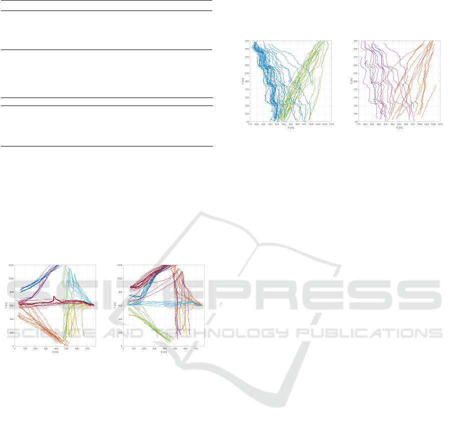
Table 3: Results of automatic model selection criteria.
Method Roundabout Circles Concentration
Unconstrained VMM 4 2 4
Constrained VMM 10 2 5
k-means 4 2 –
SSNMF (elbow/consistency) 4/5 2/3 –/–
Table 4: Influence of p on model selection in the noisy
tracks dataset. The true number of clusters is 4 and the ‘*’
indicates no clear k could be chosen.
Algorithm p = 1 p = 0.5 p = 0.1 p = 0.01 p = 10
−5
p = 0
Unconstrained VMM 4 4 4 4 9 7
Constrained VMM 7 5 5 7 10 10
k-means 4 4/5* 4/5* 4/5* 4 4
SSNMF (elbow method) 3 3 3 3/4* 4 2
SSNMF (consistency) 3 3 3 3 2 2
7.4 Real Datasets
The campus dataset is shown in Fig. 8, and is com-
posed of 134 trajectories. Since the number of clus-
ters is unknown, the methods for model selection
were executed 20 times for each k between 1 and 20.
By trial-and-error, we set p = 0.001 and 100 features
were used.
(a) 7 of the 14 clusters found
in the IST Campus dataset.
(b) The other 7 clusters.
Figure 8: The 14 clusters found in IST Campus dataset.
They are separated over 2 plots for facility of visualization.
Only the MDL minimization using the uncon-
strained VMM, which found the 14 clusters shown
in Fig. 8, gave meaningful results. For having few
parameters, MDL minimization with the constrained
VMM chooses the biggest k tested. Using the el-
bow method, on the other hand, no elbow was found
for k-means, and only a “weak” elbow was found at
k = 3 using SSNMF, but it gives meaningless clusters.
SSNMF was highly consistent for all k’s, and the only
sharp decrease happened at k = 4, which gives poor
clusters.
The staircase dataset is shown in Fig. 9. It shows a
series of people going up and down the stairs, tracked
from two different views, totaling 90 different trajec-
tories. By trial an error, p = 0.01 was found, and 50
features were used. The number of clusters was var-
ied from 1 to 12 and the tests were repeated 20 times,
to avoid bad local optima. In this case, all methods ex-
cept MDL minimization using the constrained VMM
found 4 clusters, shown in Fig. 9. This criteria failed
for not penalizing enough more complex models.
(a) 2 clusters of people going
down the stairs.
(b) The other 2 clusters, with
people going up the stairs.
Figure 9: Clusters found in the Staircase dataset.
8 CONCLUSIONS
In this work, we have presented a novel approach
to trajectory clustering, based on shape, and 3 al-
gorithms were developed for this purposed. These
methods were then tested on both synthetic and real
datasets. In both cases, all algorithms could find good
cluster assignments when given the desired number
of clusters. With model selection, the results differed
much between techniques. Overall, the best method
was MDL minimization using unconstrained VMM’s,
which found good clusters most of the time.
Possible future work includes an extension of
this methodology to 3-dimensional trajectories and an
adaptation of this methodology to clustering parts of
trajectories.
ACKNOWLEDGEMENT
This work was partially supported by FCT (Fundac¸
˜
ao
para a Ci
ˆ
encia e Tecnologia), grants PTDC/EEI-
PRO/0426/2014 and UID/EEA/5008/2013.
An extended version of this work can be found in
(Pires, 2016).
REFERENCES
Arthur, D. and Vassilvitskii, S. (2007). K-means++: The
Advantages of Careful Seeding. In Proceedings of
the Eighteenth Annual ACM-SIAM Symposium on
Discrete Algorithms, SODA ’07, pages 1027–1035,
Philadelphia, PA, USA. Society for Industrial and Ap-
plied Mathematics.
ICPRAM 2017 - 6th International Conference on Pattern Recognition Applications and Methods
80

Becker, R. A., Caceres, R., Hanson, K., Loh, J. M., Ur-
banek, S., Varshavsky, A., and Volinsky, C. (2011).
Route Classification Using Cellular Handoff Patterns.
In Proceedings of the 13th International Conference
on Ubiquitous Computing, UbiComp ’11, pages 123–
132, New York, NY, USA. ACM.
Brillinger, D., Preisler, H. K., Ager, A. A., and Kie, J. G.
(2004). An exploratory data analysis (EDA) of paths
of moving animals. In Journal of Statistical Planning
and Inference, pages 43–63.
Caner T
¨
urkmen, A. (2015). A Review of Nonnegative Ma-
trix Factorization Methods for Clustering. ArXiv e-
prints.
De Boor, C. (2001). A Practical Guide to Splines. Applied
Mathematical Sciences. Springer, Berlin.
Demirbas, M., Rudra, C., Rudra, A., and Bayir, M. A.
(2009). iMAP: Indirect measurement of air pollution
with cellphones. In Pervasive Computing and Com-
munications, 2009. PerCom 2009. IEEE International
Conference on, pages 1–6.
Dempster, A. P., Laird, N. M., and Rubin, D. B. (1977).
Maximum likelihood from incomplete data via the
EM algorithm. Journal of the Royal Statistical So-
ciety: Series B, 39(1):1–38.
Elsner, J. B. (2003). Tracking Hurricanes. Bulletin of the
American Meteorological Society, 84(3):353–356.
Ferreira, N., Klosowski, J. T., Scheidegger, C. E., and Silva,
C. T. (2012). Vector Field k-Means: Clustering Tra-
jectories by Fitting Multiple Vector Fields. CoRR,
abs/1208.5801.
Fink, D. (1997). A compendium of conjugate priors.
Fu, Z., Hu, W., and Tan, T. (2005). Similarity based vehicle
trajectory clustering and anomaly detection. In IEEE
International Conference on Image Processing 2005,
volume 2, pages II–602–5.
Gaffney, S. and Smyth, P. (1999). Trajectory Clustering
with Mixtures of Regression Models. In Proceedings
of the Fifth ACM SIGKDD International Conference
on Knowledge Discovery and Data Mining, KDD ’99,
pages 63–72, New York, NY, USA. ACM.
Hu, W., Xie, D., Fu, Z., Zeng, W., and Maybank, S. (2007).
Semantic-Based Surveillance Video Retrieval. IEEE
Transactions on Image Processing, 16(4):1168–1181.
Jain, A. K. (2010). Data Clustering: 50 Years Beyond K-
means. Pattern Recognition Letters, 31(8):651–666.
Kim, J. and Park, H. (2008). Sparse Nonnegative Matrix
Factorization for Clustering.
Lee, D. D. and Seung, H. S. (1999). Learning the parts of
objects by non-negative matrix factorization. Nature,
401:788–791.
Lee, J., Han, J., and Whang, K. (2007). Trajectory Clus-
tering: A Partition-and-Group Framework. In In SIG-
MOD, pages 593–604.
Lee, T. C. M. (2001). An Introduction to Coding Theory and
the Two-Part Minimum Description Length Principle.
International Statistical Review, 69(2):169–183.
Li, Y. and Ngom, A. (2013). The non-negative matrix fac-
torization toolbox for biological data mining. Source
Code for Biology and Medicine, 8(1):1–15.
Mardia, K. V., Hughes, G., Taylor, C. C., and Singh, H.
(2008). A Multivariate Von Mises Distribution with
Applications to Bioinformatics. The Canadian Jour-
nal of Statistics / La Revue Canadienne de Statistique,
36(1):99–109.
Nascimento, J. C., Figueiredo, M. A. T., and Marques, J. S.
(2013). Activity Recognition Using a Mixture of Vec-
tor Fields. IEEE Transactions on Image Processing,
22(5):1712–1725.
Pierobon, M., Marcon, M., Sarti, A., and Tubaro, S.
(2005). Clustering of human actions using invari-
ant body shape descriptor and dynamic time warping.
In IEEE Conference on Advanced Video and Signal
Based Surveillance, 2005., pages 22–27.
Pires, T. (2016). Shape-based Trajectory Clustering. Mas-
ter’s thesis, Instituto Superior Tcnico, Universidade de
Lisboa.
Rissanen, J. (1978). Modeling by shortest data description.
Automatica, 14(5):465 – 471.
Vlachos, M., Kollios, G., and Gunopulos, D. (2002). Dis-
covering similar multidimensional trajectories. In
Data Engineering, 2002. Proceedings. 18th Interna-
tional Conference on, pages 673–684.
Wei, J., Yu, H., Chen, J. H., and Ma, K. L. (2011). Parallel
clustering for visualizing large scientific line data. In
Large Data Analysis and Visualization (LDAV), 2011
IEEE Symposium on, pages 47–55.
Shape-based Trajectory Clustering
81
