Towards an Electronic Orientation Table: Using Features Extracted

From the Image to Register Digital Elevation Model

Léo Nicolle

, Julien Bonneton

, Hubert Konik

, Damien Muselet

and Laure Tougne

Univ. Lyon, Lyon 2, LIRIS, F-69676 Lyon, France

Univ. Lyon, UJM-Saint-Etienne, CNRS, LaHC UMR 5516, F-42023, Saint-Etienne, France

Keywords:

Skyline Detection, Digital Elevation Model, Line Matching, Color Edges.

Abstract:

Looking at a countryside, human has no difﬁculty to identify salient information such as skyline in case

of benign weather. At the same time, during the last decade, smartphones are more and more abundant in

our daily life with always new efﬁcient proposed services but augmented reality systems suffer from a lack of

performance to offer a welladapted tool in this context. Theaim of this paper is then topropose a new approach

coupling image processing and Digital Elevation Model (DEM) exploitation to remedy that shortcoming. The

proposed method ﬁrst discriminates skyline and non-skyline pixels and then introduces a realtime matching

between previously extracted map and DEM. In order to evaluate objectively each step and our ﬁnalized tool,

a new tagged dataset with ground-truth is created and will beneﬁt the entire scientiﬁc community.

1 INTRODUCTION

People hiking in the mountains or simply walking are

always looking for information about what they are

seeing : mountain names, elevations, village names,

hiking trails, tourism information, etc. Even if hiking

maps can provide such information, they require the

hiker to match the 2D data he has on the sheet with the

3D landscape he can see and this is not that always

easy for no experts. Orientation tables also help for

such problems but they are located at some too rare

points in the mountains. As nowadays everyone or al-

most has in his pocket a smartphone that integrates in-

struments such as compass, accelerometer, GPS, etc.,

with more and more memory and computing power,

the idea of this work is to create a smartphone ap-

plication that provides as much information as pos-

sible to the people looking at a mountain landscape.

The idea consists in visualizing the landscape with

the smartphone camera and the desired information

will be displayed on the screen thanks to augmented

reality tools. Objectively, some smartphone appli-

cations already provide information about mountains

peaks around a user, but the data are mostly displayed

as maps on the screen (Peakﬁnder, 2016; pointde-

vue, 2015; swissmap, 2016) or, for few of them, they

are superimposed on the screen image (Peakscanner,

2016; Peak.AR, 2010). Figure 1 shows two examples

of screenshots of such applications.

None of these applications is exploiting the im-

age content in order to help the data registration. In-

deed, the mountains peaks are reconstructed from the

available digital elevation model (DEM.) and from

the smartphone sensors (GPS and digital compasses).

The poor accuracy of such sensors badly impact the

augmented reality results, making these applications

almost unusable. This is in fact the main comments

done by the users on the stores. In recent years, many

approaches have been proposed to compensate the

lack of performance of such sensors, particularly in

constrained environment, but none our way.

Thus, we propose a new approach in order to cope

with this problem. Our solution consists in extracting

a probability map of skyline in the image acquired by

the smartphone camera and then, to match these data

with the 3D data available from the DEM. To avoid

Internet connection problems, it is directly stored in

memory before its utilization.This matching step al-

lows to display the data on the screen with high accu-

racy.

Our contributions are threefold:

• Unlike the classical skyline detection algorithms

that are based on channel-wise edge detector, we

fully exploit the 3D color information of the pixels

by learning a color metric that helps in discrim-

inating skyline edges from non-skyline edges.

Nicolle L., Bonneton J., Konik H., Muselet D. and Tougne L.

Towards an Electronic Orientation Table: Using Features Extracted From the Image to Register Digital Elevation Model.

DOI: 10.5220/0006115700280038

In Proceedings of the 12th International Joint Conference on Computer Vision, Imaging and Computer Graphics Theory and Applications (VISIGRAPP 2017), pages 28-38

ISBN: 978-989-758-227-1

Figure 1: Screenshots of two existing applications, namely

"Peakﬁnder" and "Point de vue", that display local maps on

the screen without registration.

• Because the time response and the accuracy of the

application is crucial, we propose a fast match-

ing between the probability map and the 3D data

available from the DEM.

• Since other applications exist in order to provide

information about peak mountains, we created a

new tagged dataset with ground-truth so that

the accuracy of the different approaches can be

assessed and compared. This dataset as well as

the ground-truth data will be publicly available.

2 RELATED WORKS

There is in the literature few articles dealing with the

extraction of the skyline. The purpose of some of

them is the extraction of this line from the image data

only. However others exploit the smartphone sen-

sors such as GPS and compasses in order to super-

impose the data. But the accuracy of these sensors is

small and do not have very satisfactory results from

the users point of view.

This is the reason why we recommend to exploit

the image data in order to improve the quality of the

registration step. And the main image information

that can be matched with the DEM is the skyline.

Some papers have already proposed approaches in

this direction as we shall see below but in different

contexts and with slightly different constraints.

2.1 Skyline Detection

Lie et al. (Lie et al., 2005) and Kim et al. (Byung-

Ju Kim and Kim, 2011) consider that the skyline is

constituted by the strongest edges in the image. So,

they propose ﬁrst to extract the edges with the classi-

cal Canny detector. Lie et al. apply a threshold on the

edge image to obtain a binary edge map, which is the

input of a dynamic programming search. The idea is

to connect the candidate edges that respect some cri-

teria whose aim is to preserve local smoothness and

to satisfy geometrical preferences (Lie et al., 2005).

Kim et al. propose to select the best skyline candi-

date among the output of the Canny detector as the

one that is mostly ﬂat and symmetric (Byung-Ju Kim

and Kim, 2011).

Hung et al. also apply the Canny detector as a

ﬁrst step and then learn a SVM classiﬁer on these

edge pixels to classify them into skyline edges and

no-skyline edges (Hung et al., 2013). For this clas-

siﬁcation, they are using a 210-D feature vector for

each edge pixel, that represents color and texture in-

formation extracted from the local neighborhood of

this edge pixel. At test time, they create a map for

each image in which each pixel is characterized by

a value related to its probability not to be a skyline

pixel. Then they propose a recursive algorithm that

ﬁnds the shortest path in the image, from left to right,

that minimizes the cumulative energy. This path is the

detected skyline.

Likewise, Ahmad et al. also propose to learn a

classiﬁer on the pixels in order to classify them into

skyline pixels and no-skyline pixels (Ahmad et al.,

2015). The input of the classiﬁer is a 256-D feature

vector characterizing the local neighborhood of the

considered pixel. The difference with (Hung et al.,

2013) is that they are classifying all the pixels, and not

only the edge pixels, because they argue that true sky-

line pixels may be not detected by the Canny edge de-

tector. Then each image is transformed into a classiﬁ-

cation score map which is informing about the proba-

bility of each pixel to be a skyline pixel. Finally, they

also ﬁnd the shortest path with highest cumulative en-

ergy in this map.

The approach of Saurer et al. is a bit differ-

ent from the previous ones (Saurer et al., 2016) be-

cause they classify all the pixels of the image into sky

and non-sky pixels. The feature vector characteriz-

ing each pixel is a concatenation of 4 bags of words

(textons, local ternary patterns, self-similarities and

SIFT), each one being quantized to 512 clusters and

independently in 5 different color spaces. After run-

ning the classiﬁer on all pixels of the image, they de-

termine the skyline as the line that maximizes along

the columns the number of pixels being classiﬁed as

Towards an Electronic Orientation Table: Using Features Extracted From the Image to Register Digital Elevation Model

sky above the line and as non-sky below the line, reg-

ularized by a smoothness term that helps the line to

be smooth.

The output of all these works is a binary im-

age in which each pixel is classiﬁed as skyline or

non-skyline. In order to improve the accuracy of

the matching between the DEM and our image, we

will show in the experimental results that it is better

to work with a classiﬁcation score map, where each

pixel is associated with its probability to be a sky-

line pixel, instead of a binary map (skyline vs no-

skyline). Consequently, these approaches would not

help to solve our problem as they are actually pro-

posed. Nevertheless, the classiﬁcation step of some

of them could have been interesting for our work, but

it is clear that the size of the proposed feature vectors

and their extraction time are not adapted to our prob-

lem. Indeed, we are looking for features that do not

require too much memory place and that are very fast

extracted.

Some other works also propose solutions to match

the detected 2D skyline with 3D data extracted from

the available digital elevation model.

2.2 Matching the Detected Skyline With

3D DEM Data

Baboud et al. propose a solution to automatically an-

notate mountain pictures (Baboud et al., 2011). Their

idea is to detect edges in the mountain pictures and to

match these edges with silhouettes extracted from the

3D DEM. The originality of this work is to introduce

a vector ﬁeld cross correlation that accurately match 2

sets (from image and from DEM) of local edges. Un-

fortunately, this processing can not be adapted to our

problem since it requires 2 minutes per image. In-

deed, for image annotation problems, the processing

time is not as crucial as for smartphone applications.

So they rather concentrate on accuracy matching and

do not use only the skyline in the image but all the

edges that could help for the matching.

Fedorov et al. exploit the skyline detection algo-

rithm from (Lie et al., 2005) and match this skyline

with 3D DEM data (Fedorov et al., 2014). Their aim

is also to annotate mountain pictures and so they do

not try to improve the processing time. Thus, they ap-

ply a high number of successive steps in order to im-

prove the matching. After extracting the skyline with

(Lie et al., 2005), they apply the vector ﬁeld cross cor-

relation from (Baboud et al., 2011) in order to ﬁnd 3D

skyline candidates in the DEM. Then, for each candi-

date they evaluate a Hausdorff distance with the im-

age skyline in order to ﬁnd the best candidate. Finally,

they resort to a local alignment step by applying again

vector ﬁeld cross correlations locally at different posi-

tions of the skyline. It is clear that this multiple stage

approach can not reach the processing time constraint

required by our application.

The aim of the work of Saurer et al. is to

geo-localize an image that has been acquired in the

Alps (Saurer et al., 2016). So, from an image, they

ﬁrst extract the skyline as described below and try to

ﬁnd the most similar skyline in the DEM data they

have. So their work is more about skyline retrieval

than skyline matching. Hence, they propose an in-

variant and a compact skyline descriptor and, try to

retrieve the image skyline in a dataset of skylines, in

order to deduce coarse GPS position of the consid-

ered image. Consequently, their work can not help

our skyline matching step.

Finally, Zhu et al. propose an image/DEM reg-

istration system based on skyline (Zhu et al., 2013).

This work is interesting because of its real-time con-

straint but unfortunately, it is only adapted to urban

environment and requires the presence of buildings in

the image in order to detect the vanishing point. Con-

sequently, this approach can not be used in our con-

text.

3 FAST AND ACCURATE

SKYLINE EXTRACTION AND

MATCHING WITH DEM

For our electronic orientation table, we propose a two-

steps solution. First, in a similar way as previous

works, we resort to a classiﬁcation step in order to

extract the skyline from the image. But, unlike all the

other previous approaches, we use very simple color

features that are adapted to our problem thanks to a

metric learning algorithm. Then, we propose to match

the detected skyline with the extracted skyline from

the DEM and project it in the image space.

3.1 Skyline Extraction

In order to fulﬁll our time constraints, we propose to

use the RGB data available in the image instead of

extracting some complex features. Instead of clas-

sical previous skyline detectors based on edges, we

propose to exploit the simple color difference in or-

der to detect the skyline. Of course the single color

difference is not enough to classify all the edges, but

the robustness of the approach mainly depends on

the variability of the learning data. So, during the

learning step, it is important to consider images under

a lot of different conditions (weather, illumination,

VISAPP 2017 - International Conference on Computer Vision Theory and Applications

, etc.). Evaluating accurate color differences from

uncalibrated JPEG images is not an easy task (Per-

rot et al., 2014) but our aim here is rather to eval-

uate discriminative color differences, i.e. color dif-

ferences that help to discriminate skyline edges from

non-skyline edges. For this purpose, we resort to met-

ric learning tools applied in the color RGB space.

3.1.1 Color Metric

Most of the existing works in metric learning are fo-

cused on learning a Mahalanobis-like distance be-

tween 2 vectors C

and C

in the form:

, C

) =

− C

)

M(C

− C

), (1)

where M is a positive semi-deﬁnite (PSD) matrix to

optimize (Bellet et al., 2013).

In our case, the vectors are the 3D colors denoted

by C





and C





of the two compared pixels. Let denote dk = k

− k

k ∈ {R, G, B}, the difference between the components

k of the two considered pixels. Thus the matrix M

is a 3x3 symmetric matrix such that each coefﬁcient

′

represents the weight associated to each quantity

dk.dk

′

M =









. (2)

Indeed, from eq.(1) and eq.(2), we can evaluate

, C

) as:

, C

) = m

.dR

+ m

.dR.dG+ m

.dR.dB

+ m

.dG

+ m

.dG.dB + m

.dB

(3)

Note that if M is the identity matrix, the distance d

is the simple color Euclidean distance. The aim of

metric learning is to learn the matrix M that meets the

problem constraints. In the case of skyline extraction,

we evaluate the distance between each vertical pair of

neighbor pixels and the constraint is that this distance

) have to be higher between two pixels on

both sides of the skyline than between two pixels that

are both in the sky or both in the mountain. Thus,

learning M from ground truth data (skyline vs non-

skyline edges) allows us to ﬁnd which components

are important in the color differences to discriminate

between skyline and non-skyline.

3.1.2 Learning Phase

Practically, in order to learn the 6 coefﬁcients of the

matrix M, we re-formulate the problem as a max-

margin problem and solve it with a linear SVM. In-

deed, d

, C

) can be expressed as a dot product:

, C

) =







dR.dG

dR.dB

dG.dB



















, C

) =dC

(4)

i.e. as a projection of the pair difference vector dC on

a 6D classiﬁer H

By looking at mountain landscapes it appears that

the strongest edges, despite the skyline, are mostly in

the mountains and not in the sky. So we propose to

account the edge position when detecting the skyline

so that the top edges in the image have more chance

to be classiﬁed as skyline than the bottom edges. This

is done thanks to a weighted step that is detailed in

the next paragraph. Consequently, the main aim of

our learning step is to remove the strong edges in the

sky so that the skyline appears as the ﬁrst strongest

edge in each column when visiting the pixel from top

to bottom. Thus, we create two sets of edges:

• the positive edges P

that are constituted by the

two neighbor colors that lie on both sides of the

skyline,

• the negative edges P

−

that are constituted by two

neighbor colors that lie above the positive edge of

the same column in the same image and whose eu-

clidean distance in the RGB color space is higher

than the one between the positive pair of the same

column. If in one column, no edge fulﬁlls this

condition, we randomly pick a non-skyline edge

above the positive pair of this column, so that the

positive and negative data are well balanced.

From this deﬁnition of the learning data, the aim

of our learning step is to learn the Mahalanobis ma-

trix M (or the classiﬁer H

) so that, given two

corresponding positive and negative pairs from the

same column and same image P

and P

−

, we have

) > d

−

). Thus, if the respective pair dif-

ference vectors are denoted dC

and dC

−

, we are

looking for H

so that (dC

)

> (dC

−

)

This can be done by ﬁnding the classiﬁer H

and the

bias b so that (dC

)

+b> 0 and (dC

−

)

b < 0. With a classical linear SVM, it corresponds to

maximize the margin between the two sets of pairs.

The bias is just translating all the distances, which are

initially positive, around 0, where skyline scores are

positive and non-skyline scores are negative.

Towards an Electronic Orientation Table: Using Features Extracted From the Image to Register Digital Elevation Model

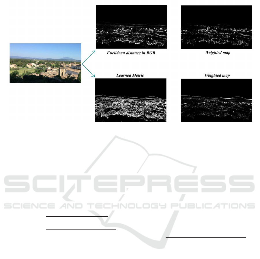
Figure 2: Comparison between the classical Euclidean distance in RGB and our color metric learning approach (see text for

details).

3.1.3 Inference

After the learning step, we get the 6 parameters of

and use them to obtain the Mahalanobis matrix M

(see eq. (2)). If this matrix is positive semi deﬁnite

(PSD), it can be decomposed thanks to the Cholesky

factorization as:

M = L

.L, (5)

where L is a 3x3 lower triangular matrix. In this case,

eq.(1) can be expressed as:

, C

) =

− C

)

.L(C

− C

)

(L.C

− L.C

)

(L.C

− L.C

(6)

which is the Euclidean distance between the two col-

ors L.C

and L.C

. Thus, from a PSD Mahalanobis

matrix M, we can deduce a matrix L that projects the

RGB colors into a new color space in which the sky-

line edges can be easily detected thanks to a simple

euclidean distance. Consequently, at test step, we just

have to project the RGB color vectors of each pixel

on the new learned discriminate color space thanks

to a simple matrix multiplication L.C

and L.C

and,

to evaluate a simple Euclidean distance between the

new colors of neighbor pixels in order to detect the

skyline. Hence, for each pixel pair, we get a distance

that is related to the chance of each edge to be on the

skyline. Note that, for all the tests we run, we always

got a matrix M that was PSD. If the matrix M is not

PSD, we have to project it on the PSD cone matrix

in order to get the nearest PSD matrix that fulﬁlls our

learning constraints.

After evaluating the Euclidean distance in the new

learned color space, we get a map of "scores" (chance

to be on the skyline), that we call the score map. Note

that, with the bias of the SVM added, the score s(i, j)

should be positive if the edge at position (i, j) is on

the skyline and negative if it is not on the skyline.

Since during the learning step, we have not consid-

ered strong edges below the skyline on each column

(we have just removed edges in the sky, not in the

mountain), we have to remove these strong edges.

Our simple but efﬁcient solution consists in weight-

ing the scores s(i, j) in the column j as follow:

sw(i, j) =

s(i, j)

∑

row=0

s(row, j)(s(row, j) > 0)

, (7)

where the row= 0 is the top row, and (s(row, j) > 0) is

a test that returns 1 if s(row, j) > 0, 1 otherwise. By

this way, we consider that, by visiting each column

from top to bottom, the ﬁrst strong positive edge has

a high chance to be on the skyline. This is due to our

learning process whose aim was to remove the strong

edges that were above the skyline.

After this step, we get a weighted-score map il-

lustrated in Figure 2. In this ﬁgure, we compare the

results obtained by our metric learning approach with

the ones obtained with the classical Euclidean dis-

tance in the RGB color space. We can see that since

the edges along the skyline are not strong in the RGB

space, they are not detected with the Euclidean dis-

tance. Fortunately, the metric we have learned clearly

identiﬁes these edges as strong ones. The images on

the right show the weighted maps obtained from ei-

ther the Euclidean distance map or from the learned

VISAPP 2017 - International Conference on Computer Vision Theory and Applications

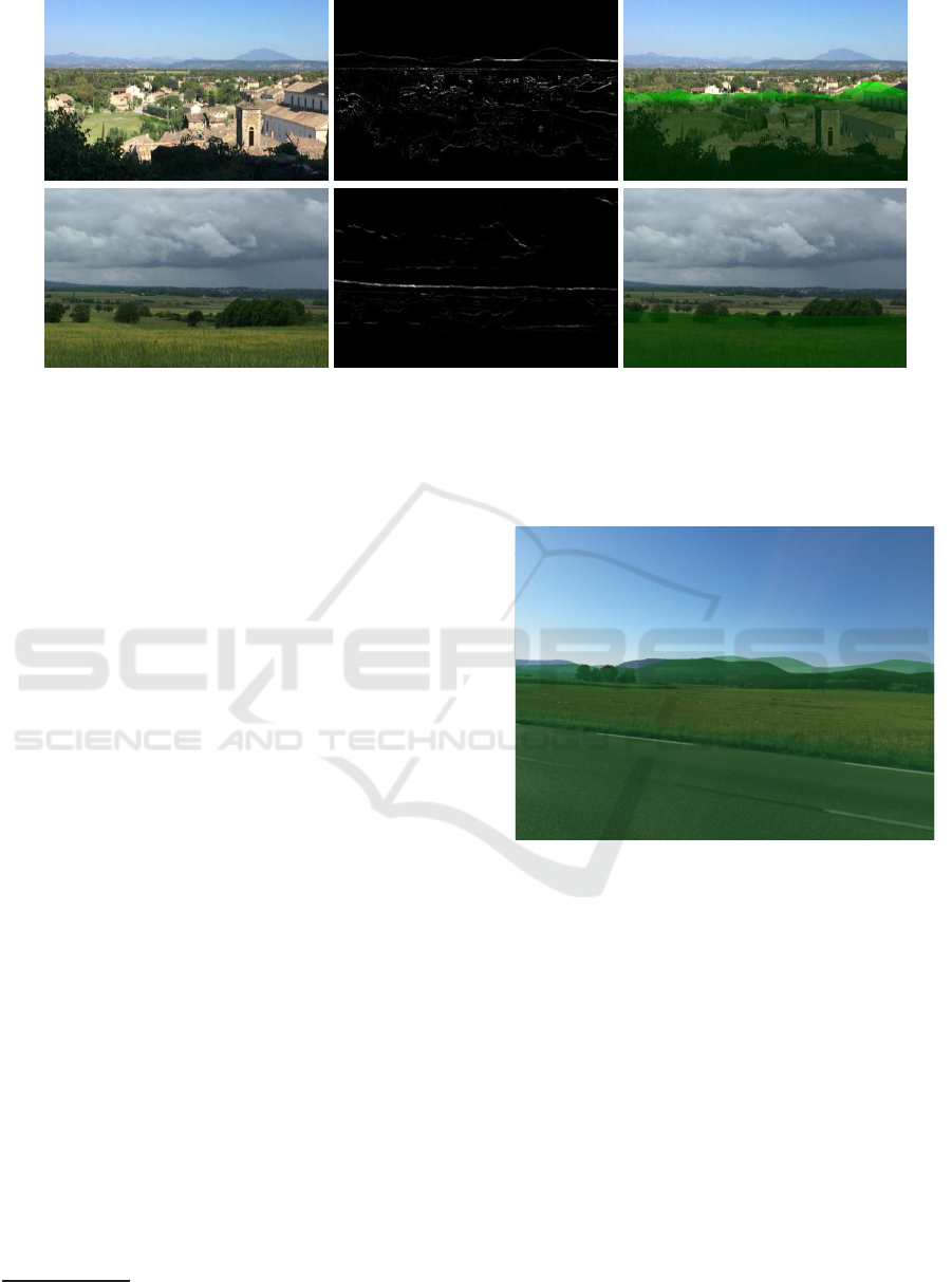
Figure 3: Two color images from our dataset along with their respective weighted color map and their relief map extracted

from DEM.

color metric. We can see that this step helps in remov-

ing most of strong edges that are below the skyline in

the color metric map.

Nevertheless, it is clear that the information pro-

vided by an image can not be sufﬁcient to get a per-

fect match between the detected pixels and the true

skyline. Consequently, after this fast color detection,

we propose to exploit the available DEM in order to

reﬁne the results. Our aim consists in registering the

DEM with the obtained weighted-score map.

3.2 Skyline Matching

Using the score map previously obtained that indi-

cates the chance for each pixel to be on the skyline,

our goal is now to register correctly the DEM on this

map. Figure 3 shows, for two images, the weighted

score maps as well as the information we have ex-

tracted from the available DEM and projected in the

2D image space from the data provided by the smart-

phone (GPS. and digital compasses) without using the

image features. In these images, the brightness of the

green is related to the altitude of the points. It is worth

mentioning that the DEM we used is free, so its res-

olution is coarse

. This ﬁgure clearly illustrates the

interest of combining the both data to detect the sky-

line: color edges and DEM.

More precisely, using the GPS coordinatesand the

intrinsic camera parameters, the DEM can be visu-

alized from the camera point of view. The ﬁgure 4

shows an example of such a visualization. But as we

can see on this ﬁgure, the projection is not perfect due

to smartphone’s measure instruments error. So let ex-

http://www.cgiar-csi.org/data/srtm-90m-digital-

elevation-database-v4-1

plain now how we can exploit the previous score map

to obtain a more reliable user’s orientation estimation.

Figure 4: Example of DEM projection, before registration

with the skyline.

Actually, such a problem is a 6-dimensional prob-

lem (considering we know camera’s intrinsic param-

eters) as explained in (Zhu et al., 2013) because the

parameters that have to be adjusted are the position

(three parameters) and the orientation (three parame-

ters too) of the camera. Trusting the GPS position and

considering the projection of the DEM onto a 2D im-

age, we reduce the problem into one that consists in

ﬁnding the best 2D transformationto match our score-

map with the DEM projection. This transformation is

composed of one 2D translation and one rotation only.

We do not have to seek for the right scale to apply to

our DEM, this information is contained into camera’s

intrinsic parameters.

In practice, we consider an angle a bit larger that

the real ﬁeld of view to deal with the lack of precision

of the compass.

Towards an Electronic Orientation Table: Using Features Extracted From the Image to Register Digital Elevation Model

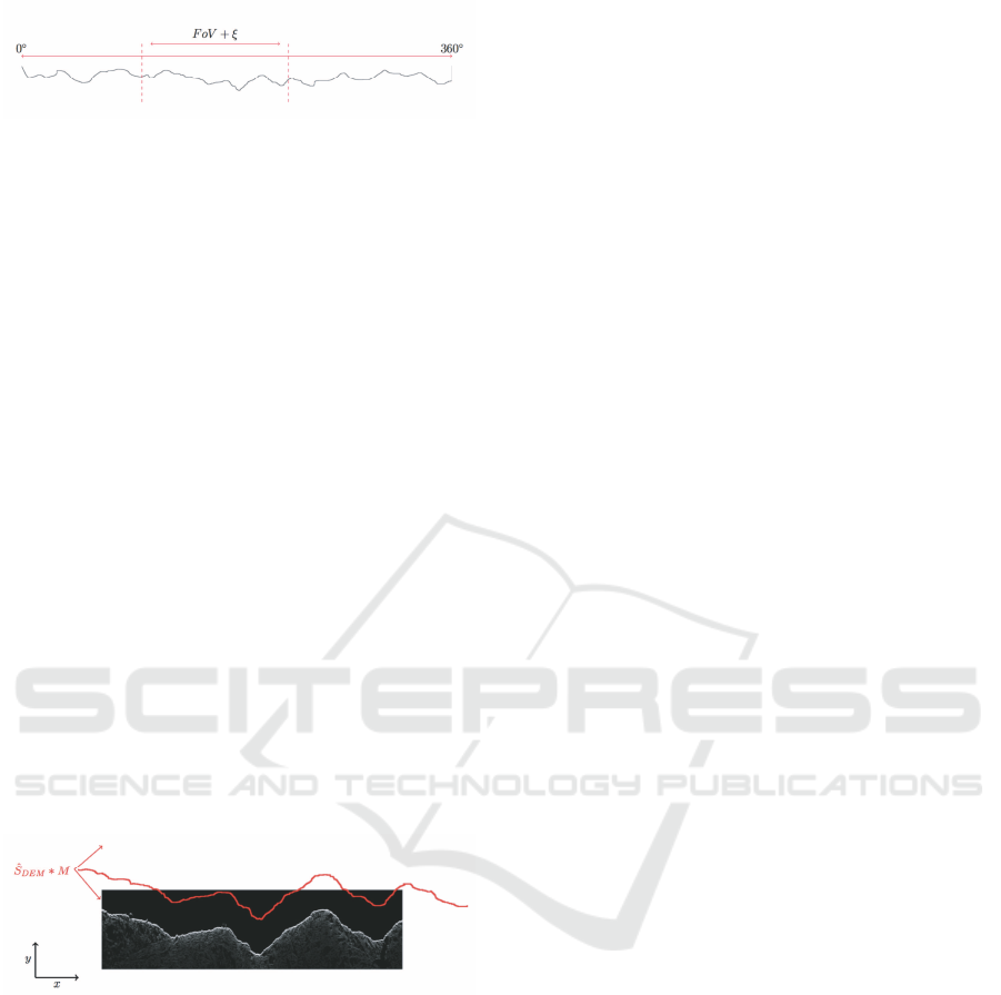
Figure 5: From the ﬁeld of view provided by the smart-

phone, we can reduce the search space.

Let us denote by S

DEM

the skyline extracted from

the projection of the DEM in the image. Notice that

to quickly perform translations and rotations, this sky-

line is stored as a set of 2D vectors, corresponding to

the relative positions of the points in the image, with

respect to the left-most point:

DEM

= {v

| v

= S

DEM

(k) − S

DEM

(0)}

where v

is the k

vector of the vectorized skyline

DEM

, and S

DEM

(i) is the 2D position of the theoreti-

cal skyline at the column i.

To ﬁnd the best registration between the DEM

skyline and the weighted-score map sw, we deﬁne the

energy function E(

DEM

, T) as follow:

DEM

, T) =

∑

k=0

sw(v

∗ M)

where T is a 3x3 matrix consisting in a translation

and a rotation and sw(p) the value of the weighted

score map at point p. The matrix M satisfying

argmax

(E(

DEM

, T)) is the best transformation to

apply to the DEM skyline to match with weighted-

score map sw (see Fig. 6).

Figure 6: Illustration of the registration between the de-

tected skyline (grey-level image) and the DEM (red curve).

In order to ﬁnd the best transform matrix T, the

brute force approach would have consist in testing all

the possible T and keeping the one that maximizes the

previous energy function E(

DEM

, T). The parame-

ters of T are the translation t

along the horizontal

axis, the translation t

along the vertical axis and the

rotation angle α around the left-most point. We call P

the set of possible solutions deﬁned as:











P = {p = (t

, α)}

∈ [t

min

; t

max

]

∈ [t

min

; t

max

]

α ∈ [α

min

; α

max

]

So, we have a 3D search space, and given our dis-

cretization choice, we have card(P) = 3.6 millions of

possible solutions to test.

In order to reduce the complexity of the algorithm,

we resort to an original multi-resolution approach.

The idea consists in:

• testing all the solutions in the search space for few

points of the skyline,

• among these solutions, keeping only the ones that

provide the top values for the energy function (the

other solutions are deﬁnitively removed from the

search space),

• adding few points to the skyline and testing the se-

lected solutions of previous step for these points,

• iterating the two previous steps until the full-

resolution skyline is tested.

Practically, we propose an algorithm in log

(n)

steps, where n is the number of points in the DEM

(close to image width), i.e. 10 steps for our 1024x768

images. At each step i, we consider only 2

points

uniformly picked in the DEM and evaluate the en-

ergy function only for these DEM points. Let de-

note u, a geometric series such that u

= card(P) and

log

(n)

= 1. So, at each step i, we keep only the u

best

transforms T that will be tested in the next step. Thus,

at each step, we reduce exponentially the number of

solutions to test while we increase the precision of the

DEM. Our matching algorithm takes 0.5 second for a

1024x768 image on a computer Intel Core i5 1.3GHz.

4 EXPERIMENTAL RESULTS

Since there is no dataset with the information required

by our system (pictures with GPS coordinates and

camera orientations), we created one which will be

publicly available. Below, we will ﬁrst present this

dataset and the necessary meta data. Then, we will

present the results on this database evaluating in par-

ticular the distance between the skyline in the ground-

truth images and the one extracted from projected

DEM in image without and with registration step.

4.1 Our Dataset

To create the dataset, we developed a smartphone ap-

plication which allows to take a picture of a landscape

and meanwhile to record the geographic position of

the user and the value of the various instruments that

are available in the smartphone. More precisely, the

data stored are the following:

• latitude, longitude, altitude,

VISAPP 2017 - International Conference on Computer Vision Theory and Applications

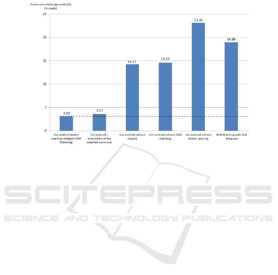
Figure 7: Average distances for the tested methods between detected and ground-truth skylines (lower is better).

• angle with north and magnetic north,

• tilts X, Y and Z.

Some of these parameters are already provided by

some datasets, but the ones concerning the orientation

of the camera are not available. All these elements are

stored in a JSON ﬁle.

Furthermore, for each acquired image, we created

a ground truth and so we manually segmented the sky-

line. Hence, JSON ﬁle is accompanied by a binary ﬁle

in which the pixels of the skyline are marked.

For the tests, about twenty images are taken into

account. We will enrich the dataset over time.

4.2 Results

In order to assess the quality of our algorithm, we pro-

pose to test it on our dataset and to evaluate the aver-

age distance (in pixels) over all the images between

the skyline we obtain and the ground-truth skyline.

Of course this distance is relative to the image size

1024x768. The results are shown in ﬁgure 7.

In order to check the relevance of each contribu-

tion of our algorithm, we have run several tests by

removing each single step from the whole process

and check the results for each. We recall that the

main contributions of our algorithm are : color metric

learning, score weighting and matching with DEM.

In ﬁgure 7, we clearly see the relevance of each in-

dividual step, since the average distance dramatically

increases (from 3 pixels to 14 or even 23) when we

remove one of them. It is worth mentioning that our

learning step has been run on the CH1 dataset de-

scribed in (Saurer et al., 2016) and not on our dataset.

The CH1 dataset consists of images of mountains in

which the skyline has been manually segmented (un-

fortunately, no geographic information are provided

with this dataset, so that we can not extract the cor-

rect DEM to run our algorithm on these images). This

showsthat our newcolor metric has been learned once

on one dataset and can be used on any other dataset

without ﬁne-tuning it to the new considered images.

Furthermore, in ﬁgure 7, we show the results ob-

tained by our algorithm when the score map is bi-

narized before the DEM matching. The binarization

consists in only keeping the highest score in each col-

umn. We can see that this binarization does not help

the matching step (and even slightly increases the dis-

tance). This is interesting to see that our matching al-

gorithm is performing better with a dense score map

(where each pixel is characterized by a score) than

with a binary skyline detection. Finally, we also show

the results provided by a baseline method which con-

sists in evaluating column-wise the RGB distances in

the image and to match the DEM with this score map

(without weights and without ad-hoc color metric).

Figure 7 shows that this approach provides poor re-

sults since the average distance between the detected

and the ground-truth skylines is around 18 pixels.

We can see that by combining all our contribu-

tions, we obtain an average distance equals to 3 pix-

els, which is negligible with respect to the size of the

images (0.4 %) . This shows that the proposed sky-

Towards an Electronic Orientation Table: Using Features Extracted From the Image to Register Digital Elevation Model

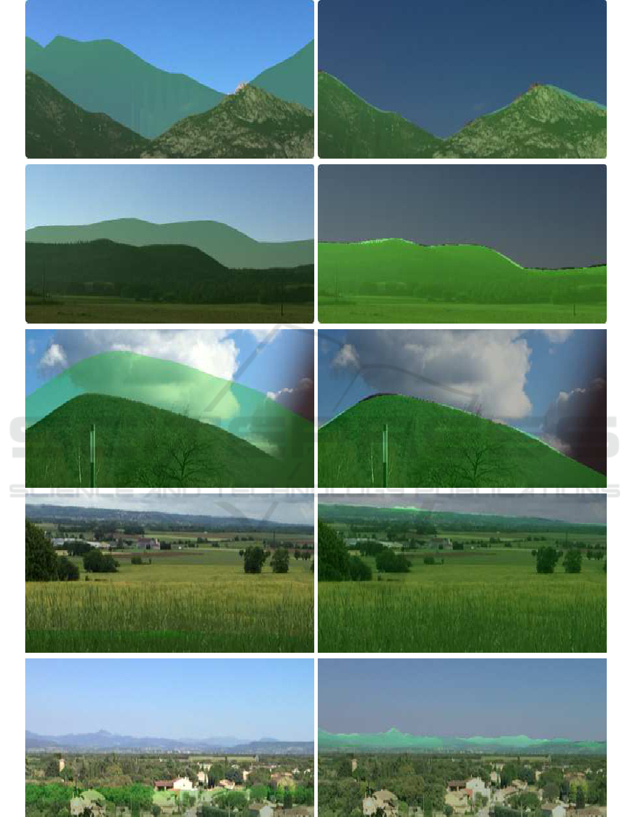
Figure 8: Some results provided by our method. Left : DEM. projection from the smartphone sensors. Right : DEM.

projection after registration with our weigthed score map.

VISAPP 2017 - International Conference on Computer Vision Theory and Applications

line detection is the perfect candidate to be integrated

in an electronic orientation table.

In ﬁgure 8, there are some visual results. We have

zoomed on some examples of mountains to show in

detail the obtained registration. The two original reg-

istrations using only the DEM and the smartphone lo-

calization objectively completely fail but the result is

better by coupling DEM and image processing.

5 CONCLUSION

This paper presented a robust two-steps method able

to create a smartphone application identifying instan-

taneously the skyline in an image. The proposed

method starts by image simpliﬁcation based on efﬁ-

cient color difference between aligned pixels giving

rise to a score map between sky and non-sky pix-

els. Then, based on available data directly from the

smartphone offering a coarse localization, a second

step matches extracted skylines from the digital ele-

vation model with this map to identify precisely the

real skyline. The interest of this couple between im-

age processing and digital elevation model is twofold:

it gives an efﬁcient tool in this context of electronic

orientation table, and it allows to improve augmented

reality tools based on smartphones using image pro-

cessing techniques. Moreover,the tagged dataset built

in this paper will beneﬁt the entire community in

this ﬁeld. Future works will ﬁrst consist in analyz-

ing robustness to meteorologic conditions and then in

detecting other notable elements in the image using

image analysis but also the DEM. Let us remember

that our ﬁnal goal is to present to the user informa-

tion concerning points of interest in the image using

augmented reality. For this, we also intend to use

databases containing monuments, roads, etc.

There is still an immense potential in this ﬁeld be-

cause of its utility in many areas like in tourism of

course but also, for example, for hikers who want to

visualize hiking trails, for persons interested in geol-

ogy because it would be possible to show them the

structure of the ground also and so on. Smartphones

are today abundant in our daily life and augmented

reality systems could be developed by mixing their

instruments with image processing algorithms.

ACKNOWLEDGEMENT

The authors acknowledge the support from Le Pro-

gramme Avenir Lyon Saint-Etienne Image et Percep-

tion Embarquées (PALSE IPEm – ANR-11-IDEX-

0007). They also would like to thank Thierry Joliveau

for his help in this work.

REFERENCES

Ahmad, T., Bebis, G., Nicolescu, M., Neﬁan, A., and Fong,

T. (2015). An edge-less approach to horizon line de-

tection. 2015 IEEE 14th International Conference on

Machine Learning and Applications (ICMLA), pages

1095–1102.

Baboud, L.,

Cadík, M., Eisemann, E., and Seidel, H.-P.

(2011). Automatic photo-to-terrain alignment for the

annotation of mountain pictures. In Proceedings of the

2011 IEEE Conference on Computer Vision and Pat-

tern Recognition, Washington, DC, USA. IEEE Com-

puter Society.

Bellet, A., Habrard, A., and Sebban, M. (2013). A survey

on metric learning for feature vectors and structured

data (arxiv:1306.6709v3). In Tech. report.

Byung-Ju Kim, Jong-Jin Shin, H.-J. N. and Kim, J.-S.

(2011). Skyline extraction using a multistage edge ﬁl-

tering. International Journal of Electrical, Computer,

Energetic, Electronic and Communication Engineer-

ing.

Fedorov, R., Fraternali, P., and Tagliasacchi, M. (2014).

Mountain peak identiﬁcation in visual content based

on coarse digital elevation models. Proceedings of

the 3rd ACM International Workshop on Multimedia

Analysis for Ecological Data, pages 7–11.

Hung, Y.-L., Su, C.-W., Chang, Y.-H., Chang, J.-C., and

Tyan, H.-R. (2013). Skyline localization for mountain

images. In 2013 IEEE International Conference on

Multimedia and Expo (ICME), pages 1–6.

Lie, W.-N., Lin, T. C. I., Lin, T.-C., and Hung, K.-S. (2005).

A robust dynamic programming algorithm to extract

skyline in images for navigation. Pattern Recogn.

Lett., 26(2):221–230.

Peak.AR (2010). http://peakar.salzburgresearch.at/. Ac-

cessed: 2016-09-05.

Peakﬁnder (2016). https://www.peakﬁnder.org. Accessed:

2016-09-05.

Peakscanner (2016). http://www.peakscanner.com/. Ac-

cessed: 2016-09-05.

Perrot, M., Habrard, A., Muselet, D., and Sebban, M.

(2014). Modeling perceptual color differences by lo-

cal metric learning. In European Conference on Com-

puter Vision (ECCV), pages 96–111. Springer Interna-

tional Publishing.

pointdevue (2015). https://itunes.apple.com/fr/app/

point-de-vue/id341554913?mt=8. Accessed: 2016-

09-08.

Saurer, O., Baatz, G., Köser, K., Ladický, L., and Pollefeys,

M. (2016). Image based geo-localization in the alps.

Int. J. Comput. Vision, 116(3):213–225.

swissmap (2016). https://itunes.apple.com/fr/app/

swiss-map-mobile/id311447284?mt=8. Accessed:

2016-09-08.

Towards an Electronic Orientation Table: Using Features Extracted From the Image to Register Digital Elevation Model

Zhu, S., Morin, L., Pressigout, M., Moreau, G., and

Servières, M. (2013). Video/gis registration system

based on skyline matching method. In 2013 IEEE

International Conference on Image Processing, pages

3632–3636.

VISAPP 2017 - International Conference on Computer Vision Theory and Applications