
Restoration of Temporal Image Sequence
from a Single Image Captured by a Correlation Image Sensor
Kohei Kawade
1
, Akihiro Wakita
1
, Tastuya Yokota
1
, Hidekata Hontani
1
and Shigeru Ando
2
1
Computer Science and Engineering, Nagoya Institute of Technology, Gokiso-cho, Showa-ku,
Nagoya-shi, Aichi 466-8555, Japan
2
Richo Elemex Corporation, 3-69, Ida-cho, Okazaki-shi, Aichi, 444-8586, Japan
Keywords:
Optical Flow, Correlation Image Sensor.
Abstract:
We propose a method that restores a temporal image sequence, which describes how a scene temporally
changed during the exposure period, from a given still image captured by a correlation image sensor (CIS).
The restored images have higher spatial resolutions than the original still image, and the restored temporal
sequence would be useful for motion analysis in applications such as landmark tracking and video labeling.
The CIS is different from conventional image sensors because each pixel of the CIS can directly measure the
Fourier coefficients of the temporal change of the light intensity observed during the exposure period. Given
a single image captured by the CIS, hence, one can restore the temporal image sequence by computing the
Fourier series of the temporal change of the light strength at each pixel. Through this temporal sequence
restoration, one can also reduce motion blur. The proposed method improves the performance of motion blur
reduction by estimating the Fourier coefficients of the frequencies higher than the measured ones. In this
work, we show that the Fourier coefficients of the higher frequencies can be estimated based on the optical
flow constraint. Some experimental results with images captured by the CIS are demonstrated.
1 INTRODUCTION
Each pixel in a traditional image sensor measures the
temporal integration of light strength over an expo-
sure time. Because of the temporal integration, the
measured pixel value does not contain information
of the temporal change of the light strength gener-
ated during the exposure time. Moving objects or
moving cameras generate the temporal change of the
light strength, but a traditional camera fails to record
this temporal change and hence restoring the tempo-
ral change from a given still image is difficult. In this
article, we propose a method that restores the tempo-
ral image sequence, which describes how the image
temporally changed during the exposure period, from
a given still image captured by a correlation image
sensor (CIS)(Ando et al., 1997)(Ando and Kimachi,
2003)(Wei et al., 2009)(Hontani et al., 2014). Several
methods have been proposed for motion estimation
or for temporal change restoration from a single im-
age mainly because a single still image does not have
enough information for restoring temporal changes.
As described above, the proposed method cap-
tures an image by using a CIS. Each pixel of a CIS
measures not only a temporal integration of the light
strength but also a temporal correlation between the
light strength and a reference temporal signal supplied
from the outside of the CIS to each pixel during an
exposure period. By using sinusoidal functions as the
references, one can measure a set of the Fourier coef-
ficients of the light strength at each pixel. These mea-
surements of the Fourier coefficients include the in-
formation on the temporal change of the light strength
during the exposure period and it was reported that the
CIS made a problem of the optical flow computation
well-posed(Wei et al., 2009). The proposed method
restores the temporal change of the image intensity at
each pixel by using the measured Fourier coefficients:
Just by computing the Fourier series of the tempo-
ral change at each pixel, one can approximately re-
store the temporal change of the image. The method
improves the accuracy of the approximation by us-
ing other information obtained though optical flow
computation. The temporal change approximately re-
stored by the Fourier series is always periodic, but this
is not always true. In other words, if one restores the
temporal change of the light intensity only by using
the Fourier series, the restored light intensity at the
Kawade K., Wakita A., Yokota T., Hontani H. and Ando S.
Restoration of Temporal Image Sequence from a Single Image Captured by a Correlation Image Sensor.
DOI: 10.5220/0006115301810191
In Proceedings of the 12th International Joint Conference on Computer Vision, Imaging and Computer Graphics Theory and Applications (VISIGRAPP 2017), pages 181-191
ISBN: 978-989-758-227-1
Copyright
c
2017 by SCITEPRESS – Science and Technology Publications, Lda. All rights reserved
181

beginning of the exposure period is always the same
as the intensity at the end of the period. The proposed
method thus improves the accuracy by explicitly esti-
mating the difference between the light intensity at the
beginning and that at the end of the exposure period
through optical flow computation as will be described
later. The proposed method can restore an instanta-
neous image that describes the spatial distribution of
the light intensity on the image sensor corresponding
to an arbitrary point of time during the exposure time.
The restored instantaneous image should have motion
blur less than the given original image. Our proposed
method has strong relationships with methods used
for motion blur reduction. The authors are interested
in the comparison of the performance of the motion
blur reduction between the proposed method and the
other existing methods, but the comparison is out of
the scope of this article. One of the strong points of
the proposed method is that it restores a series of im-
ages with higher spatial resolution, which represents
the temporal change of the images during the shutter
is open. In the next section, we describe methods of
temporal change restoration and of blind motion de-
blurring, which can be interpreted as the restoration of
the instantaneous image that describes the light inten-
sity at some specific point of time during the exposure
period.
2 RELATED WORK
Several methods that can restore the temporal change
of the light strength during the exposure time have
been proposed. To the best of our knowledge, all
those methods employ an active sensing strategy:
A coded light, which is synchronized with the tim-
ing of the camera shutter, is used when a still im-
age is captured and the temporal change of the light
strength is decoded by a temporal high-frequency pat-
tern of the shutter (Kadambi et al., 2013)(Velten et al.,
2013)(Heide et al., 2013). Such a camera can mea-
sure the depth in realtime and can restore the tempo-
ral change of the light strength during the exposure
time. In contrast to these methods, our method em-
ploys a passive sensing strategy: No encoded light
that is specific to the camera used is required.
From the view point of the passive sensing strat-
egy, the proposed method has strong relationships
with methods for blind motion deblurring. One can
divide the methods of the nonuniform blind deblur-
ring into two classes: In one class, a given image is
captured by a traditional image sensor. In the other
class, a nontraditional sensor is used for capturing
the image. The majority of the methods in the for-
mer class employ a Bayesian framework for remov-
ing motion blurs. These methods combine natural
image priors(Levin, 2006)(Fergus et al., 2006)(Shan
et al., 2008)(Cho and Lee, 2009)(Cai et al., 2012)(Xu
et al., 2013)(Deshpande and Patnaik, 2014), blurring
kernel priors(Jia, 2007)(Shan et al., 2008)(Cho and
Lee, 2009)(Xu and Jia, 2010)(Cai et al., 2012)(Xu
et al., 2013), or models of motions(Jia, 2007)(Shan
et al., 2007)(Whyte et al., 2012), and optimization
techniques to recover both the blurring kernel and the
deblurred latent image simultaneously.
The natural image priors include distribution mod-
els of spatial gradient magnitudes(Field, 1994)(Fer-
gus et al., 2006)(Shan et al., 2008) and sparse rep-
resentations based on local appearances(Deshpande
and Patnaik, 2014) or on the gradients(Shan et al.,
2008)(Xu and Jia, 2010)(Cai et al., 2012). The
blurring kernel priors play important roles especially
when the motion blurs result from camera shakes.
For example, a motion density function(Gupta et al.,
2010), spatially sparse local filter(Fergus et al., 2006),
camera geometry model(Whyte et al., 2012), and
framelet-based sparse representation(Cai et al., 2012)
are introduced as the kernel priors. Object motion
estimation is useful for removing motion blurs(Jia,
2007), and a parametric motion descriptor(Shan et al.,
2007) is used for the estimation from a single given
image. The proposed method also estimates optical
flow from a single given image and uses it for remov-
ing motion blurs.
In the former class, nontraditional image sensors
are used for obtaining the additional information use-
ful for motion deblurring. Hybrid cameras(Nayar and
Ben-Ezra, 2004)(Tai et al., 2010), which detect cam-
era motion using data from a video camera attached
to a still camera, are used for motion deblurring. In-
ertial measurement sensors are also used for the esti-
mation of camera motion(Joshi et al., 2010). Among
the methods in this class, the proposed method is most
similar to the motion deblurring methods using coded
exposure photography(Raskar et al., 2006)(Agrawal
and Raskar, 2009)(McCloskey et al., 2012). Control-
ling the camera’s shutter open and close during the ex-
posure period with a binary pseudo-random sequence,
one obtains a broad-band motion blurring kernel that
preserves high-frequency spatial details. Combining
the estimation of objects’ motions, one can estimate
the blurring kernel and compute the latent nonblurred
image by deconvoluving the given motion blurred im-
age with the estimated kernel.
In coded exposure photography, the camera en-
codes the temporal change of incident light strength
at each pixel during the exposure period with the bi-
nary pseudo-random shutter pattern. A CIS used in
VISAPP 2017 - International Conference on Computer Vision Theory and Applications
182

the proposed method, on the other hand, encodes the
temporal change with analog sinusoidal reference sig-
nals. As will be described later, a CIS has three chan-
nels each of which encodes the temporal change with
a different reference signal and makes the problem of
optical flow computation well-posed. The proposed
method first computes the optical flow of a given sin-
gle image and then uses the optical flow for restoring
higher frequency components of the temporal change
of the light strength during the exposure period.
The contributions of this study are as follows: (1)
A completely passive method is proposed for restor-
ing the temporal change of the light strength during
the exposure period from a single still image captured
by a CIS, (2) To improve the quality of the restored
images, a method is proposed for computing the tem-
poral frequency components that are higher than those
of the reference signals, and (3) It is shown that the
restoration can reduce motion blur.
3 CORRELATION IMAGE
SENSOR (CIS)
Let exposure time be denoted by T and let the time
during which the shutter is open be denoted by t,
where 0 ≤ t ≤ T . Let the coordinates on an image
sensor be denoted by x = (x, y)
|
and let f (t,x) denote
the strength of the incident light that comes from the
lens system to the pixel at location x at time t. The
location variable, x, is often omitted as f (t) = f (t,x)
when the location is clearly known from the context.
The CIS used in this study has three channels and
a pixel value of the s-th channel (s ∈ {1,2,3}) denotes
the temporal correlation between the light strength,
f (t, x), and a reference signal, r
s
(t), which is supplied
from the outside of the CIS to all pixels as
I
s
(x) =
∫
T
0
f (t, x)r
s
(t)dt.
Let r
s
(t) = cos(nω
0
t + 2(s − 1)π/3) + 1/3 where
ω
0
= 2π/T and n ∈ Z. Then, we can mea-
sure the following three values at each pixel si-
multaneously(Ando et al., 1997)(Ando and Kimachi,
2003)(Wei et al., 2009) as follows:
g
0
(x) =
1
T
∫
T
0
f (t, x)dt, (1)
g
n,R
(x) =
1
T
∫
T
0
f (t, x)cos(nω
0
t)dt, (2)
and
g
n,I
(x) =
1
T
∫
T
0
f (t, x)sin(nω
0
t)dt, (3)
where g
n,R
(x) and g
n,I
(x) are the real and imaginary
parts of a complex Fourier coefficient g
n
that corre-
sponds to the frequency n/T . It should be noted that
no image sensor can measure the light strength f (t,x)
directly and traditional image sensors can measure
only g
0
(x). In this manuscript, we set n = 1 and a CIS
sensor measures g
0
(x) and g
1
(x) = g
1,R
(x)+ jg
1,I
(x),
where j is the unit imaginary number.
3.1 Optical Flow Computation with a
CIS
We can compute an optical flow v(x) = (v
x
(x),v
y
(x))
|
from a single image measured by the CIS. In the com-
putation, we assume that the light strength arriving
from each point of an object is invariant with respect
to time and that the following equation is satisfied
when the shutter is open, t ∈ [0,T ]:
d
dt
f (t, x) =
v
x
∂
∂x
+ v
y
∂
∂y
+
∂
∂t
f (t, x) = 0. (4)
Integrating (4) over the exposure time with a weight
e
− jnω
0
t
/T where n ∈ Z, we obtain the following equa-
tion:
0 =
1
T
∫
T
0
v
x
∂
∂x
+ v
y
∂
∂y
+
∂
∂t
f (t,x)e
− jnω
0
t
dt
=
1
T
∫
T
0
v
x
∂
∂x
+ v
y
∂
∂y
f (t,x)e
− jnω
0
t
+
∂
∂t
f (t,x)e
jnω
0
t
dt
=
v
x
∂
∂x
+ v
y
∂
∂y
g
n
(x)
+
1
T
[ f (t, x)e
jnω
0
t
]
T
0
+ jnω
0
∫
T
0
f (t,x)e
jnω
0
t
dt
=
v
x
∂
∂x
+ v
y
∂
∂y
g
n
(x) +F
0
(x) + jnω
0
g
n
(x),
(5)
where
g
n
(
x
)
is an image of the Fourier coefficients of
temporal signals f (t,x) such that
g
n
(x) =
1
T
∫
T
0
f (t, x)e
− jnω
0
t
d t (6)
and F
0
denotes the difference of the boundary val-
ues such that F
0
(x) = [ f (t,x)]
T
0
/T = { f (T,x) −
f (0,x)}/T .
As described above, a CIS can measure both g
0
(x)
and g
1
(x) at each pixel. Substituting n = 0 and n = 1
to (5), we obtain two different equations. Eliminat-
ing the variable F
0
from these two equations, we can
derive a linear complex equation as follows:
v
x
∂
∂x
+ v
y
∂
∂y
{
g
1
(x) − g
0
(x)
}
+ jω
0
g
1
(x) = 0.
(7)
Equation (7) consists of two real coefficient equations
and we can derive the following linear equation of v:
Av = d, (8)
Restoration of Temporal Image Sequence from a Single Image Captured by a Correlation Image Sensor
183

where d = [ω
0
g
1,I
,−ω
0
g
1,R
]
T
and
A =
∂
x
{g
1,R
+ g
0
} ∂
y
{g
1,R
+ g
0
}
∂
x
g
1,I
∂
y
g
1,I
. (9)
One can estimate v(x) by solving the linear equation
shown in (8). It should be noted that the problem of
optical flow computation is well-posed when one cap-
tures images with a CIS though the problem is ill-
posed when one captures images with a traditional
image sensor. The added measurements, g
n
(x), can
introduce extra information that constrains the solu-
tion.
Substituting n = 0 and n = 1 to (5), we obtain the
following two equations:
v
x
∂
∂x
+ v
y
∂
∂y
g
0
(x) + F
0
(x) = 0, (10)
v
x
∂
∂x
+ v
y
∂
∂y
g
1
,
R
(x) + F
0
(x) − ω
0
g
1,I
= 0. (11)
Solving the system of linear equations (10) and (11),
we can obtain the following equation.
F
0
(x) = −
1
2
v
x
∂
∂x
+ v
y
∂
∂y
(g
1,R
(x) + g
0
(x))
+
ω
0
2
g
1,I
(x). (12)
Once we compute the flow v(x), the difference of the
boundary values F
0
(x) can be estimated by solving
(12). The values, v
x
, v
y
, and F
0
, computed at each
pixel are used in the restoration process described in
the next section.
4 RESTORATION OF
TEMPORAL CHANGE OF
LIGHT STRENGTH DURING
EXPOSURE PERIOD
The objective is to restore the temporal change of the
strength of light strength, f (t,x) (0 ≤ t ≤ T ), at each
pixel from the measurements, g
0
(x) and g
1
(x), ob-
tained by a CIS. It is not difficult to approximately
restore f (t, x) by using the N-th order Fourier series
expansion of f (t) = f (t,x) (N ∈ N) such that
˜
f
N
(t) =
N
∑
n=−N
g
n
e
jnω
0
t
, (13)
where g
n
(n ∈ Z) are the Fourier coefficients as de-
fined in (6). As g
−n
= g
∗
n
holds when f (t) is a real
function, the original signal f (t) can be approximated
by using the Fourier coefficients g
0
and g
1
measured
by a CIS as follows:
˜
f
1
(t) =
1
∑
n=−1
g
n
e
jnω
0
t
= g
0
+ 2Re[g
1
e
jω
0
t
], (14)
where Re[c] denotes the real part of a complex num-
ber c. The proposed method restores f (t) by improv-
ing the approximation
˜
f
1
(t) by restoring (i) the differ-
ence of the boundary values f (T ) − f (0), and (ii) the
higher frequency components g
n
(n > 1) that are not
measured by the CIS.
4.1 Restoration of Boundary Values
˜
f
N
(0) and
˜
f
N
(T ) approximate f (0) and f (T ) inaccu-
rately in general.
˜
f
N
(0) =
˜
f
N
(T ) always holds be-
cause
˜
f
N
(t) shown in (13) is a linear combination
of e
jnω
0
t
(n = 0,1,. .. ,N) that are all periodic func-
tions with period T . It leads to
˜
F
0
(x) = {
˜
f
N
(T ) −
˜
f
N
(0)}/T = 0, which is not always consistent with
the true value of F
0
. The value of
˜
f
N
(t) changes ex-
tremely rapidly near the boundaries t = 0 and t = T .
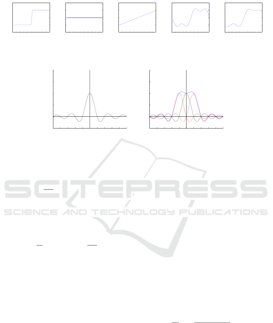
The left panel of Fig.1 shows examples of the signals
restored by g
n
(n = 1,2,. .. ). A true and unobservable
signal f (t), where f (T ) ̸= f (0), is shown at the top of
Fig.1. As N increases, the resultant
˜
f
N
(t) converges to
the original one, but we can notice that
˜
f
N
(T ) =
˜
f
N
(0)
is always satisfied and can see the rapid change near
the measurement boundaries t = 0 and t = T .
The proposed method compensates for the rapid
changes by adding a new function s(t) to
˜
f
N
(t) so that
the resultant function
ˆ
f
N
(t) =
˜
f
N
(t) + s(t) is consis-
tent with the value of F
0
estimated by using (12) and
with the Fourier coefficients g
n
(x) that are measured
(or would be computed) from f (t, x). The consistency
with respect to the Fourier coefficients requires s(t) to
satisfy the following equation:
∫
T
0
˜
f
N
(t)e
− jnω
0
t
d t =
∫
T
0
ˆ
f
N
(t)e
− jnω
0
t
dt. (15)
This leads to
∫
T
0
s(t)e
− jnω
0
t
dt = 0. (16)
Substituting n = 0, we notice that s(t) must be anti-
symmetric with respect to the reflection at the center
time of the exposure period t = T /2. Among the anti-
symmetric functions, we select the following equation
because it is consistent with the value of F
0
:
s(t) = s
N
(t) = F
0
(t − T /2) +
∑
N
n=1
a
n
sin(nω
0
t)
T
,
(17)
which always satisfies s
N
(T )−s
N
(0) = F
0
. The coef-
ficients proposed in (17), a
n
, are scalar and their val-
ues should be determined so that
ˆ
f
N
(t) is consistent
VISAPP 2017 - International Conference on Computer Vision Theory and Applications
184
0 0.1 0.2 0.3 0.4 0.5 0.6 0.7 0.8 0.9 1
−0.5
0
0.5
1
1.5
TIME
f (t)
0 0.1 0.2 0.3 0.4 0.5 0.6 0.7 0.8 0.9 1
−0.5
0
0.5
1
1.5
TIME
(a)
˜
f
0
(t)
0 0.1 0.2 0.3 0.4 0.5 0.6 0.7 0.8 0.9 1
−0.5
0
0.5
1
1.5
TIME
(b)
ˆ
f
0
(t)
0 0.1 0.2 0.3 0.4 0.5 0.6 0.7 0.8 0.9 1
−0.5
0
0.5
1
1.5
TIME
(c)
˜
f
3
(t)
0 0.1 0.2 0.3 0.4 0.5 0.6 0.7 0.8 0.9 1
−0.5
0
0.5
1
1.5
TIME
(d)
ˆ
f
3
(t)
Figure 1: Examples of the approximations. An original signal f (t), the Fourier approximations
˜
f
N
(t) shown in (13), and the
modified approximation
ˆ
f
N
(t) in (19) are indicated.
−5 −4 −3 −2 −1 0 1 2 3 4 5
−0.5
0
0.5
1
1.5
2
Frequency [1/vT]
(A)
−5 −4 −3 −2 −1 0 1 2 3 4 5
−0.5
0
0.5
1
1.5
2
Frequency [1/vT]
(B)
Figure 2: (A) A graph of H
0
along the direction of v. (B) Graphs of H
0
(black), H
1
(red), and H
∗
1
(red). H
1
improves the
bandwidth of the resultant filter (blue).
with g
n
(n ≥ 1). Solving (16) with respect to a
n
, we
get
a
n
=
2
nω
0
, (n = 1, 2,. ..,N). (18)
As a result, the proposed method restores the latent
image by using the following equation:
ˆ
f
N
(t,x) = g
0
(x) + 2
N
∑
n=1
Re[g
n
(x)e
jnω
0
t
]
+
F
0
T
(t − T /2) +
N
∑
n=1
2
nω
0
sin(nω
0
t)
.
(19)
(a) and (c) of Fig.1 show examples of
ˆ
f
N
(t) that ap-
proximate f (t), which is a step function in this exam-
ple. Comparing (b) and (d) of Fig.1 respectively, we
observe that the rapid changes near the measurement
boundaries are suppressed.
4.2 Restoration of Higher Frequency
Components
The number of channels of a CIS is limited to three
and we use them for measuring the lower temporal
frequency components of f (t). Restoring the higher
temporal frequency components of f (t, x), one can re-
store higher spatial frequency components of f (t, x)
and can deblur the motion-blurred gray-scale image
g
0
(x) more crisply. As will be described later, one can
restore the higher temporal frequency components of
f (t, x) by using (5). Before the restoration algorithm
is described, the relationships between the temporal
frequencies of f (t) = f (t, x) and the spatial frequen-
cies of g
n
(x) are discussed.
4.2.1 Spatial Motion Blur in Fourier Coefficient
Image
Let the velocity of a moving target in an image be
denoted by v = (v
x
,v
y
)
|
= v(cosθ,sin θ)
|
, where v
denotes the speed and θ denotes the angle between
v and the x-axis. The motion blur generated on
the gray-scale image g
0
(x) by the target motion can
be represented by a spatial convolution with a one-
dimensional box filter h
0
(x) that averages the inten-
sities along a line segment of length vT , which is a
trajectory of the moving target:
g
0
(x) = f (x) ∗ h
0
(x), (20)
where ∗ denotes a spatial convolution,
h
0
(x) =
1
vT
rect
x cosθ + ysin θ
vT
δ(v
|
⊥
x), (21)
v
⊥
denotes a unit vector perpendicular to v,
rect(x) =
1, if |x| ≤ 1/2,
0, otherwise,
(22)
and f (x) = f (t = T /2,x). We fix the time to the center
of the exposure time t = T /2 for avoiding the effects
of the temporal boundaries of the measurements.
Restoration of Temporal Image Sequence from a Single Image Captured by a Correlation Image Sensor
185
¯
f (1,x)
¯
f (15,x)
¯
f (30,x)
g
0
(x)
g
1,R
(x)
g
1,I
(x)
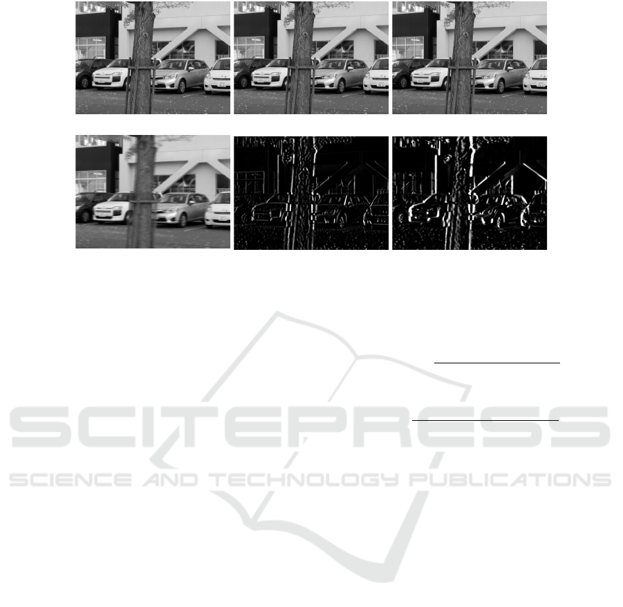
Figure 3: Top: Examples of the still images
¯
f (k, x). Bottom: Generated images, g
0
(x), g
1,R
(x), and g
1,I
(x).
A motion blur generated on the complex Fourier
coefficient image g
n
(x) by the target motion can be
represented by a spatial convolution with a differ-
ent one-dimensional filter h
n
(x). Let x = vt de-
note the location of the moving target in the image,
where the origin of the coordinate system is tem-
porarily set to the target’s location at t = 0. Then,
multiplying v
|
from the left, we obtains the equa-
tion t = v
|
x/v
2
= (v
x
cosθ + v
y
sinθ)/v. Substituting
this equation and ω
0
= 2π/T into the representation
of the reference temporal signal, e
jnω
0
t
, we obtain a
spatial filter that corresponds to the reference signal
e
2π jn(v
x
cosθ+v
y
sinθ)/vT
. The profile of this spatial filter
along the trajectory of the moving target is a complex
sinusoidal curve with frequency n/vT . Multiplying
this spatial filter with h
0
, we get h
n
(x), where
h
n
(x) = h
0
(x)e
2π jn(xcosθ+ysinθ)/vT
, (23)
and this spatial filter generates the Fourier coefficient
image, g
n
(x), as given by the following equation:
g
n
(x) = f (x) ∗ h
n
(x). (24)
Let the spatial Fourier transformation of f (x) be
denoted by F(u), where u = (u
x
,u
y
)
|
denotes the
two-dimensional spatial frequency and let the Fourier
transformation of
˜
f
1
(x) in (14) be denoted by
˜
F
1
(u).
We can now derive the following equation from (14)
˜
F
1
(u) = F(u)
{
H
0
(u) + H
1
(u) + H
∗
1
(−u)
}
, (25)
where H
n
(u) denotes the Fourier transformation of
h
n
(x) and is given as
H
n
(u) = H
0
(u) ∗ δ(u
x
cosθ+ u
y
sinθ+ n/vT ), (26)
where ∗ is now a convolution with respect to the
frequencies. The Fourier transformation of the one-
dimensional box filter, h
0
(x), is given as a sinc func-
tion such that
H
0
(u) =
sin(π(T v
x
u
x
+ T v
y
u
y
))
π(T v
x
u
x
+ T v
y
u
y
)
. (27)
Finally, we obtain
H
n
(u) =
sin(π(T v
x
u
x
+ T v
y
u
y
+ n))
π(T v
x
u
x
+ T v
y
u
y
+ n)
. (28)
Figure 2 shows the profiles of H
0
and of H
1
along a
line parallel to the motion direction. As shown by the
profile of H
0
, h
0
is a low-pass filter and generates the
spatial motion blur of a moving target in g
0
(x). The
graph of H
n
is obtained by shifting that of H
0
by n
toward the motion direction and h
n
is a band-pass fil-
ter of which the spatial center frequency is n/vT . The
approximation
ˆ
f
1
(x) shown in (19) is computed with
g
0
and g
1
and the latter measurement g
1
improves the
spatial bandwidth by adding the two band-pass filters
H
1
and H
∗
1
to the low-pass filter H
0
as shown in (25).
It should be noted that one can increase the band-
width of the restoration and can obtain crisper images
if one can estimate the higher frequency components
g
n
(x) (n > 1) and approximates as follows:
˜
f
N
(t,x) =
N
∑
n=−N
g
n
(x)e
jnω
0
t
, (29)
where N ≥ 1. The bandwidth of
˜
f
N
(t) is wider than
that of
˜
f
1
(t) when N ≥ 1 and the restoration accuracy
is improved by the addition of g
n
(n ≥ 1). The method
for the estimation of g
n
(x) is described next.
4.2.2 Estimation with Sparsity Regularization
The proposed method estimates g
n
(x) (n > 1) by us-
ing (5). As mentioned above, the values of v
x
(x),
VISAPP 2017 - International Conference on Computer Vision Theory and Applications
186
g
0
(x)
ˆ
f
3
(t = 0)
ˆ
f
3
(t = 7/30)
ˆ
f
3
(t = 15/30)
ˆ
f
3
(t = 22/30)
g
0
(x)
v(x)
F
0
(
x
)
ˆ
f
3
(t = 0)
ˆ
f
3
(t = T /3)
ˆ
f
3
(t = 2T /3)
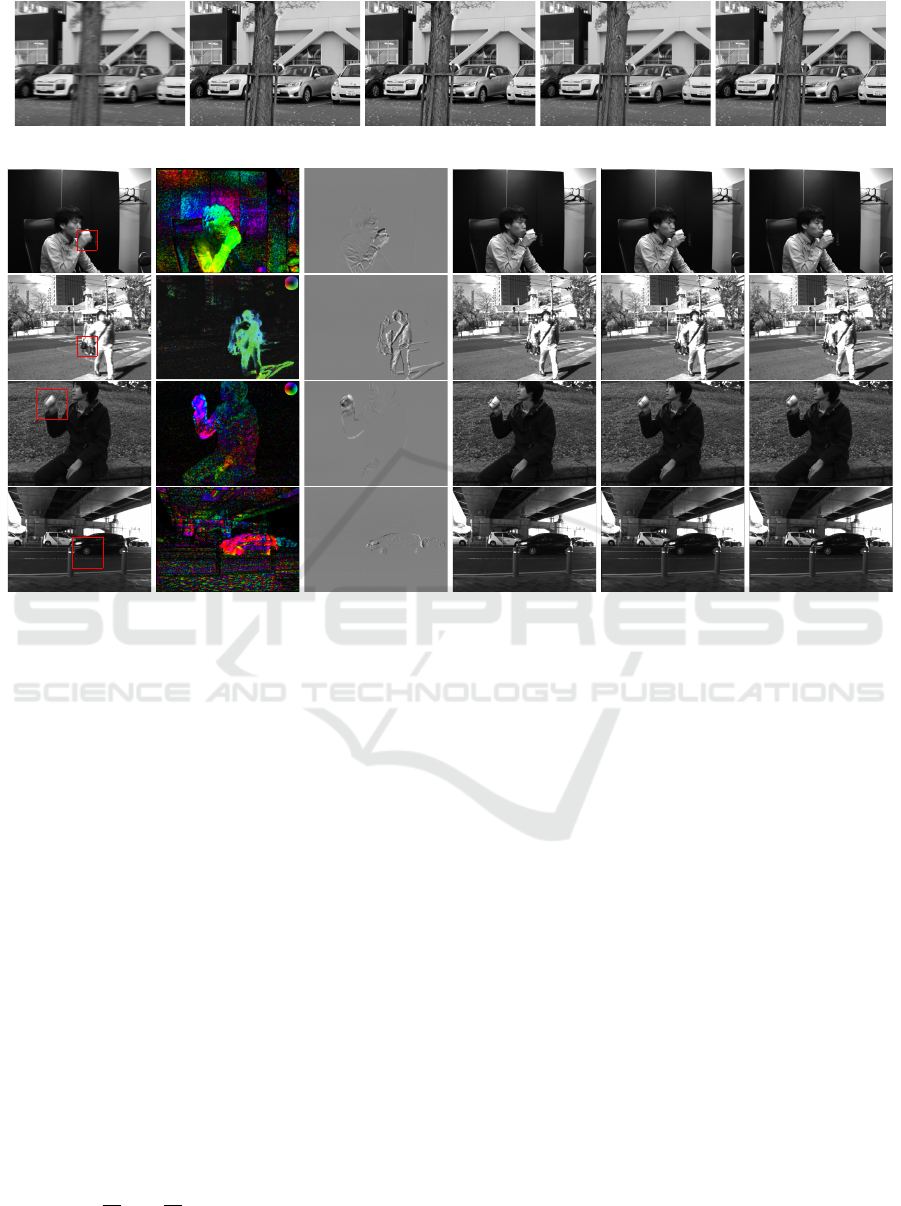
Figure 4: Top row: g
0
(x) artificially generated from M = 30 still images shown in Fig.3 and
ˆ
f
3
(t,x) for each t. The Second to
Bottom rows: g
0
(x) measured by a CIS and the results, v(x), F
0
(x), and
ˆ
f
3
(t,x), computed from the images captured by the
CIS.
v
y
(x), and F
0
(x) can be estimated by using the mea-
sured values of g
0
(x) and g
1
(x). No other measure-
ments are needed for the estimation. Once these val-
ues are estimated, g
n
(x) is the only unknown variable
in the linear complex equation shown in (5) and one
can estimate its value by solving the equation.
These estimated values, though, can be inaccurate
especially when the differential equation (5) does not
hold as some irregular events like occlusions or spec-
ular reflections occur. We need a robust estimation
method that automatically detects and excludes data
that do not obey an employed model. Assuming that
the regions in which the equation (5) does not hold
are sparse in a given image, the proposed method uses
a regularization technique proposed in (Ayvaci et al.,
2012) for making the estimation robust against such
irregulars.
Let e(x) denote a residual of the right hand side of
(5) defined as
e(x)
.
=
v
x
∂
∂x
+ v
y
∂
∂y
g
n
(x) + F
0
(x) + jnω
0
g
n
(x).
(30)
Let D denote the entire image domain and let Ω de-
note subregions in D in which (5) does not hold. We
assume that the residual e(x) obeys a normal distribu-
tion with zero mean and small variance, if x ∈ D \ Ω,
where (5) is satisfied. If x ∈ Ω, on the other hand,
(5) is not satisfied and the residual, e(x), can have an
arbitrary value, ρ(x).
Let e(x) = e
1
(x) + e
2
(x) such that
e
1
(x) =
ρ(x), x ∈ Ω,
0, x ∈ D \ Ω,
(31)
and
e
2
(x) =
0, x ∈ Ω,
N (x), x ∈ D \ Ω,
(32)
where N denotes a variable that obeys the normal dis-
tribution. Then, e
1
is large and sparse, and e
2
is small
and dense. Based on the discussion above, the pro-
posed method minimizes the following cost function:
J
n
(g
n
,e
1
) = ∥e
2
∥
L
2
(D)
+ α∥e
1
∥
L
1
+ β∥g
n
(x)∥
L
2
,
=
∥
(v
|
∇)g
n
+ F
0
+ jnω
0
g
n
− e
1
∥
L
2
(D)
+ α∥e
1
∥
L
1
+ β∥g
n
∥
L
2
(33)
Restoration of Temporal Image Sequence from a Single Image Captured by a Correlation Image Sensor
187
0 0.005 0.01 0.015 0.02 0.025 0.03 0.035
0
50
100
150
200
250
f (t, x
left
)
0 0.005 0.01 0.015 0.02 0.025 0.03 0.035
0
50
100
150
200
250
ˆ
f
1
(t,x
left
)
0 0.005 0.01 0.015 0.02 0.025 0.03 0.035
0
50
100
150
200
250
ˆ
f
3
(t,x
left
)
0 0.005 0.01 0.015 0.02 0.025 0.03 0.035
0
50
100
150
200
250
f (t, x
middle
)
0 0.005 0.01 0.015 0.02 0.025 0.03 0.035
0
50
100
150
200
250
ˆ
f
1
(t,x
middle
)
0 0.005 0.01 0.015 0.02 0.025 0.03 0.035
0
50
100
150
200
250
ˆ
f
3
(t,x
middle
)
0 0.005 0.01 0.015 0.02 0.025 0.03 0.035
0
50
100
150
200
250
f (t, x
right
)
0 0.005 0.01 0.015 0.02 0.025 0.03 0.035
0
50
100
150
200
250
ˆ
f
1
(t,x
right
)
0 0.005 0.01 0.015 0.02 0.025 0.03 0.035
0
50
100
150
200
250
ˆ
f
3
(t,x
right
)
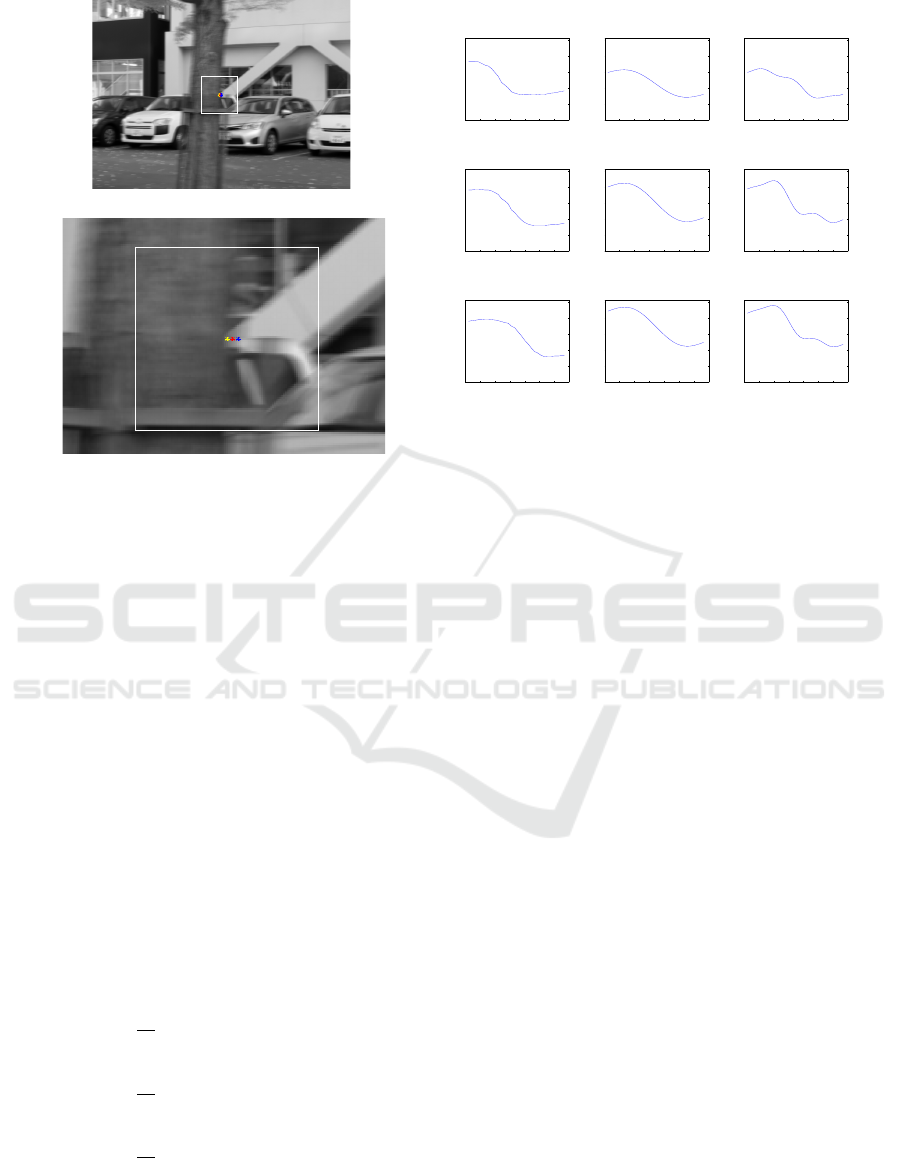
Figure 5: Left Panel: The location of three pixels indicated by three dots (yellow (x
left
), red (x
middle
). Right Panel: Examples
of f (t = (k − 1)/M) (left column),
ˆ
f
N=1
(t) (middle column), and
ˆ
f
N=3
(t) (right column) at the three pixels.
where α and β are positive scalar coefficients for the
regularization terms and their values are experimen-
tally determined. J
n
(g
n
,e
1
) is convex with respect to
g
n
and e
1
when v and F
0
are fixed and then one can
obtain the unique solution of g
n
(x) and e
1
(x).
5 EXPERIMENTAL RESULTS
The performance was evaluated with sets of simulated
data and with images captured by a CIS.
5.1 Experiments with Simulated Data
Sets of M still images of a stationary scene,
{
¯
f (k,x)|k = 1, 2,..., M}, were captured by a slowly
translating traditional camera for simulating f (t,x)
(0 ≤ t < 1) and artificially generated g
0
(x) and g
1
(x)
from each of the sets as follows:
g
0
(x) =
1
M
M
∑
k=1
¯
f (k,x), (34)
g
1,R
(x) =
1
M
M
∑
k=1
¯
f (k,x) cos(2π(k − 1)/M),(35)
g
1,I
(x) =
1
M
M
∑
k=1
¯
f (k,x) sin(2π(k − 1)/M). (36)
Figure 3 shows examples of
¯
f (k,x) (M = 30) and
the corresponding g
0
(x) and g
1
(x). One can see
the motion blurs in g
0
(x). The top row in Fig. 4
shows g
0
(x) again and some restored latent images,
ˆ
f
3
((k − 1)/M,x) (k = 0,7, 15,22). Comparing with
g
0
(x) shown in the left, we can see that the proposed
method suppressed the motion blur in g
0
(x) and re-
stored the temporal change of the light strength during
the exposure time by computing
ˆ
f
3
(t,x). Examples of
the true signal f (t = (k − 1)/M,x) and the restored
signals
ˆ
f
N
(t,x) at three neighboring pixels are shown
in Fig.5. The locations of the three pixels are shown
at the left panel in the figure. They were located near
the right boundary of a tree, which moved toward the
right. The left column in the right panel shows the true
profiles of f (t, x) at the three points x
left
, x
middle
, and
x
right
. The value of f decreased rapidly when the tree,
which moved from left to right in the image, reached
to each pixel. The graphs in the middle column and in
the right column show the restored temporal change
of the light strength at each pixel with N = 1 (mid-
dle column) and with N = 3 (right column) as shown
in (19), respectively. The latent true signals f (t, x) in
the left column were smooth enough and no higher
frequency components were required for describing
the true signal. Hence,
ˆ
f
1
(t,x), which consists of only
lower frequency components, approximated the latent
signal more accurately than
ˆ
f
3
(t,x), in which one can
see some artifacts like aliasing. It is included in our
future works to adaptively determine the appropriate
value of N in (19) for each pixel.
VISAPP 2017 - International Conference on Computer Vision Theory and Applications
188
g
0
(x)
ˆ
f
3
(t = 0, x)
ˆ
f
3
(T /3,x )
ˆ
f
3
(2T /3,x )
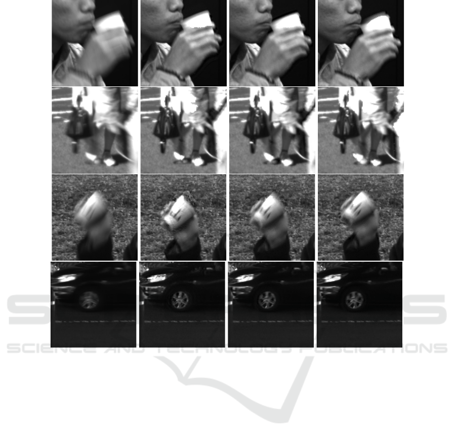
Figure 6: Enlarged parts of the images shown in Fig.4
5.2 Experiments with Images Captured
by a CIS
A set of images was captured by the CIS, and the im-
age size was 512 × 704, with the exposure time set
as T = 1/30 s. Examples of g
0
(x) are shown at the
leftmost panels in the second to bottom rows of Fig.4.
Firstly, solving the linear equation (8), we computed
the flow v, and the difference of the boundary values
F
0
(x) for each image. Examples of the obtained re-
sults are shown in Fig.4. As shown, F
0
(v) had nonzero
values around the regions corresponding to the mo-
tion blurs. Then, minimizing J(g
n
,e
1
) in (33), the
method computed g
n
(x) (n = 2, 3) and e
1
. Using the
estimated values of g
n
(n = 2, 3) with the measured
values, g
0
and g
1
, the method restored images
ˆ
f
3
(t,x)
as shown in the middle and the bottom rows in Fig.4.
Enlarged parts of the images, g
0
(x) and
ˆ
f
3
(t,x), are
shown in Fig.6. Comparing with g
0
(x) at the leftmost
panel, we can see that the restored images include less
motion blurs.
6 SUMMARY AND FUTURE
WORK
We proposed a CIS-based method that removes mo-
tion blurs from a single image and restores the la-
tent temporal images, which represent the temporal
change of the light strength during the exposure pe-
riod. We believe that our proposed method would
largely improve the stability and accuracy of motion
analysis including landmark tracking or optical flow
computation that are crucial in medical image analy-
sis.
One advantage of the proposed method is found
especially in the restoration of the latent temporal im-
ages. The restoration of the temporal change of the
light strength during the exposure time from a single
given image is very difficult when the image is cap-
Restoration of Temporal Image Sequence from a Single Image Captured by a Correlation Image Sensor
189

tured with a traditional image sensor. On the other
hand, a CIS modulates the temporal change of the
light strength at each pixel with the sinusoidal refer-
ence signals and records the temporal change with its
Fourier coefficients. Using these coefficients, one can
compute optical flow, v(x), and the difference of the
boundary values, F
0
(x), from a single image captured
by a CIS. Once one obtains v(x) and F
0
(x), one can
restore the higher temporal frequency components,
g
n
(x) (n ≥ 2), based mainly on the optical flow con-
straint, which represents the temporal invariance of
the strength of an incident light coming from an ob-
ject point.
The biggest limitation of the proposed method is
that the optical flow constraint (5) used in the pro-
posed method assumes that a flow observed at each
pixel, v(x), is constant with respect to time during
the exposure time. This is not true especially when
the motion blurs are generated with a high-frequency
motion such as a hand shake. Many blind motion de-
blurring methods can estimate spatial blurring kernels
from a single blurred image by introducing the prior
knowledge on natural images and/or on kernels. The
future works would include the use of the strategies
employed by those blind motion deblurring methods
for estimating the spatial blurring kernels that are con-
sistent not only with the blurred image g
0
(x) but also
with the Fourier coefficient image, g
1
(x), so that one
can restore more accurate and crisp images that rep-
resent the temporal change during the exposure time.
REFERENCES
Agrawal, A. and Raskar, R. (2009). Optimal single image
capture for motion deblurring. In Computer Vision
and Pattern Recognition, 2009. CVPR 2009. IEEE
Conference on , pages 2560–2567. IEEE.
Ando, S. and Kimachi, A. (2003). Correlation im-
age sensor: Two-dimensional matched detection of
amplitude-modulated light. Electron Devices, IEEE
Transactions on, 50(10):2059–2066.
Ando, S., Nakamura, T., and Sakaguchi, T. (1997). Ul-
trafast correlation image sensor: concept, design,
and applications. In Solid State Sensors and Actu-
ators, 1997. TRANSDUCERS’97 Chicago., 1997 In-
ternational Conference on, volume 1, pages 307–310.
IEEE.
Ayvaci, A., Raptis, M., and Soatto, S. (2012). Sparse occlu-
sion detection with optical flow. International Journal
of Computer Vision, 97(3):322–338.
Cai, J.-F., Ji, H., Liu, C., and Shen, Z. (2012). Framelet-
based blind motion deblurring from a single image.
Image Processing, IEEE Transactions on, 21(2):562–
572.
Cho, S. and Lee, S. (2009). Fast motion deblurring. In
ACM Transactions on Graphics (TOG), volume 28,
page 145. ACM.
Deshpande, A. M. and Patnaik, S. (2014). Uniform and non-
uniform single image deblurring based on sparse rep-
resentation and adaptive dictionary learning. The In-
ternational Journal of Multimedia & Its Applications
(IJMA), 6(01):47–60.
Fergus, R., Singh, B., Hertzmann, A., Roweis, S. T., and
Freeman, W. T. (2006). Removing camera shake from
a single photograph. ACM Transactions on Graphics
(TOG), 25(3):787–794.
Field, D. J. (1994). What is the goal of sensory coding?
Neural computation, 6(4):559–601.
Gupta, A., Joshi, N., Zitnick, C. L., Cohen, M., and Cur-
less, B. (2010). Single image deblurring using motion
density functions. In Computer Vision–ECCV 2010,
pages 171–184. Springer.
Heide, F., Hullin, M. B., Gregson, J., and Heidrich, W.
(2013). Low-budget transient imaging using photonic
mixer devices. ACM Transactions on Graphics (ToG),
32(4):45.
Hontani, H., Oishi, G., and Kitagawa, T. (2014). Local es-
timation of high velocity optical flow with correlation
image sensor. In Computer Vision–ECCV 2014, pages
235–249. Springer.
Jia, J. (2007). Single image motion deblurring using trans-
parency. In Computer Vision and Pattern Recogni-
tion, 2007. CVPR’07. IEEE Conference on, pages 1–
8. IEEE.
Joshi, N., Kang, S. B., Zitnick, C. L., and Szeliski, R.
(2010). Image deblurring using inertial measurement
sensors. In ACM Transactions on Graphics (TOG),
volume 29, page 30. ACM.
Kadambi, A., Whyte, R., Bhandari, A., Streeter, L., Barsi,
C., Dorrington, A., and Raskar, R. (2013). Coded
time of flight cameras: sparse deconvolution to ad-
dress multipath interference and recover time profiles.
ACM Transactions on Graphics (TOG), 32(6):167.
Levin, A. (2006). Blind motion deblurring using image
statistics. In Advances in Neural Information Process-
ing Systems, pages 841–848.
McCloskey, S., Ding, Y., and Yu, J. (2012). Design and esti-
mation of coded exposure point spread functions. Pat-
tern Analysis and Machine Intelligence, IEEE Trans-
actions on, 34(10):2071–2077.
Nayar, S. K. and Ben-Ezra, M. (2004). Motion-based mo-
tion deblurring. Pattern Analysis and Machine Intelli-
gence, IEEE Transactions on, 26(6):689–698.
Raskar, R., Agrawal, A., and Tumblin, J. (2006). Coded
exposure photography: motion deblurring using flut-
tered shutter. ACM Transactions on Graphics (TOG),
25(3):795–804.
Shan, Q., Jia, J., and Agarwala, A. (2008). High-quality mo-
tion deblurring from a single image. In ACM Transac-
tions on Graphics (TOG), volume 27, page 73. ACM.
Shan, Q., Xiong, W., and Jia, J. (2007). Rotational motion
deblurring of a rigid object from a single image. In
Computer Vision, 2007. ICCV 2007. IEEE 11th Inter-
national Conference on, pages 1–8. IEEE.
VISAPP 2017 - International Conference on Computer Vision Theory and Applications
190

Tai, Y.-W., Du, H., Brown, M. S., and Lin, S. (2010).
Correction of spatially varying image and video mo-
tion blur using a hybrid camera. Pattern Analy-
sis and Machine Intelligence, IEEE Transactions on,
32(6):1012–1028.
Velten, A., Wu, D., Jarabo, A., Masia, B., Barsi, C., Joshi,
C., Lawson, E., Bawendi, M., Gutierrez, D., and
Raskar, R. (2013). Femto-photography: capturing and
visualizing the propagation of light. ACM Transac-
tions on Graphics (TOG), 32(4):44.
Wei, D., Masurel, P., Kurihara, T., and Ando, S. (2009).
Optical flow determination with complex-sinusoidally
modulated imaging. relation, 7(8):9.
Whyte, O., Sivic, J., Zisserman, A., and Ponce, J. (2012).
Non-uniform deblurring for shaken images. Interna-
tional journal of computer vision, 98(2):168–186.
Xu, L. and Jia, J. (2010). Two-phase kernel estimation for
robust motion deblurring. In Computer Vision–ECCV
2010, pages 157–170. Springer.
Xu, L., Zheng, S., and Jia, J. (2013). Unnatural l0 sparse
representation for natural image deblurring. In Com-
puter Vision and Pattern Recognition (CVPR), 2013
IEEE Conference on, pages 1107–1114. IEEE.
Restoration of Temporal Image Sequence from a Single Image Captured by a Correlation Image Sensor
191
