Proposal of New Tracer Concentration Model in Lung PCT Study

Comparison with Commonly Used Gamma-variate Model

Maciej Browarczyk

, Renata Kalicka

and Seweryn Lipiński

Department of Biomedical Engineering, Gdańsk University of Technology, Narutowicza 11/12 Street, Gdańsk, Poland

Department of Electrical Engineering, Power Engineering, Electronics and Automation,

University of Warmia and Mazury, Olsztyn, Poland

Keywords: Modelling, pCT, Gamma-Variate, Gauss, Rayleigh.

Abstract: Perfusion computed tomography (pCT) is one of the methods that enable non-invasive imaging of the

hemodynamics of organs and tissues. On the basis of pCT measurements, perfusion parameters such as

blood flow (BF), blood volume (BV), mean transit time (MTT) and permeability surface (PS) are calculated

and then used for quantitative evaluation of the tissue condition. To calculate perfusion parameters it is

necessary to approximate concentration-time curves using regression function. In this paper we compared

three regression functions: first commonly used gamma-variate function, second and third Gauss and

Rayleigh functions, not previously used for this purpose. The Gauss function showed clear advantage over

the others when considering results of simulated data analysis. Actual measurements analysis confirmed

conclusions from simulated data analysis. It was showed that contrary to widely accepted belief, the

differences between rising and falling edge slope angles of concentration-time curves are inconsiderable.

For that reason, it can be assumed that rising and falling edges are symmetrical. The main conclusion is that

the Gauss function gives a more robust fit than the widely used gamma-variate function when modelling

concentration-time curves in lung pCT studies.

1 INTRODUCTION

Perfusion computed tomography (pCT) is one of the

methods that enable non-invasive imaging of the

hemodynamics of organs and tissues. On the basis of

pCT measurements, perfusion parameters such as

blood flow (BF), blood volume (BV), mean transit

time (MTT) and permeability surface (PS) are

calculated and then used for quantitative evaluation

of the tissue condition. Usefulness of perfusion

parameters has been proved in the diagnosis of brain

(Wintermark et al., 2008), kidneys (Zhao et al.,

2010), liver (Mírka et al., 2010), pancreas

(Balthazar, 2011) and spleen (Sauter et al., 2012). In

the case of lungs, as in other organs, perfusion

imaging is particularly useful for diagnosing cancer

(Cao, 2011). The method allows not only for

establishing the tumour size and location (Nakano et

al., 2013), but may also provide important predictive

information concerning tumour vasculature (Ng and

Goh, 2010). Lung pCT measurements can also help

in the diagnosis of diabetic pulmonary

microangiopathy (Browarczyk et al., 2015; Kalicka

et al., 2015).

The pCT chest technique uses the intravenous

injection of a non-iodinated contrast agent (tracer)

and the sequential scanning of the chest when the

agent passes through the lungs for the first time

("first-pass"). The tissue concentration-time curve

c(t) is obtained for every pixel of the diagnosed

cross-section. The relationship between the arterial

input function tracer concentration c

AIF

(t) on

entering the region of interest (ROI) and the c(t)

measured within the ROI has been formulated on the

basis of the tracer kinetics theory.

To calculate perfusion parameters it is necessary

to approximate the data in the form of c(t) and c

AIF

(t)

measurements with regression function. The most

commonly used functions for this purpose are the

gamma-variate (Blomley and Dawson, 1997;

Jackson, 2004) and two- or three-exponential

functions (Kalicka and Pietrenko-Dąbrowska, 2007;

Srikanchana et al., 2004). However, regression

functions that have good properties when applied to

dynamic brain research (Kalicka and Pietrenko-

Dąbrowska, 2007) or carotid artery (Lampaskis et

al., 2009), demonstrate worse performance, for

instance, in the case of renal studies (Balvay et al.,

134

Browarczyk M., Kalicka R. and LipiÅ

Dski S.

Proposal of New Tracer Concentration Model in Lung PCT Study - Comparison with Commonly Used Gamma-variate Model.

DOI: 10.5220/0006115101340140

In Proceedings of the 10th International Joint Conference on Biomedical Engineering Systems and Technologies (BIOSTEC 2017), pages 134-140

ISBN: 978-989-758-212-7

2008) or liver (Lampaskis et al., 2009). This

observation inspired us to compare the gamma-

variate function with the Gauss and the Rayleigh

functions in pCT lung studies. The Gauss and the

Rayleigh functions were not previously used for this

purpose. All of the functions were compared using

both actual and simulated pCT data.

2 MATERIAL AND METHODS

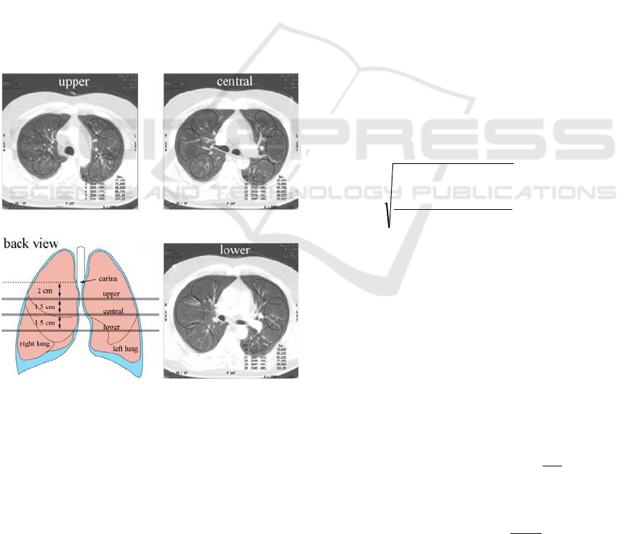
The clinical measurements were performed on a 64-

row Light Speed VCT CT scanner produced by GE

Healthcare USA. Pulmonary perfusion was axially

evaluated in three cross-sections: the upper, the

middle and the lower parts of the lungs (2 cm, 3.5

cm and 5 cm below carina, respectively, see figure

1), 12 s after the intravenous administration of 40 ml

a non-iodinated contrast medium at a rate of 4 ml/s.

Each of the three sequences consists of 89 scans,

with a resolution of 512 at 512 pixels, collected with

a sampling interval of 1 s.

Figure 1: Three cross-sections obtained from healthy

subject.

Two data sets were collected. The first data set

consists of actual measurements and the second data

set was simulated. Simulated data were used for

extended analysis of error propagation for all

considered regression functions. Each data set, both

measured and simulated, consists of three

concentration-time curves, one per lung region:

arterial input function (AIF), blood vessels and

parenchyma. The first data set was created from the

actual measurements obtained from 5 healthy

subjects, 2 females and 3 males, aged 33-67. The

second data set was simulated using the actual

measurements obtained from another healthy subject

(female, 67 y/o, non-smoking with no diagnosed

acute or chronic diseases affecting pulmonary

functions). All patients received written information

about the study, then gave written consent to

participate. The study was approved by the

Independent Commission on Bioethics Committee

for Scientific Research at the Medical University of

Gdańsk.

The simulations were conducted in the following

way: 100 pixels were manually chosen from the

upper, the central and the lower cross-sections. The

selected pixels provide j=1,...,100 concentration-

time curves c

). Each curve consists i=1,...,89

measurements. The most typical concentration-time

curve c

typ

) was calculated as a mean vector,

defined as sum of vectors c

) divided by number of

vectors. The typical curves were used to perform

100 simulation runs c

sim









typsim ii

tcGtc



(1)

G(c

typ

),R) is the random numbers generator of the

normal distribution with mean parameter c

typ

) and

standard deviation R equal to the residual variance

of actual measurements:

 



100,

typ









tctc

iji

(2)

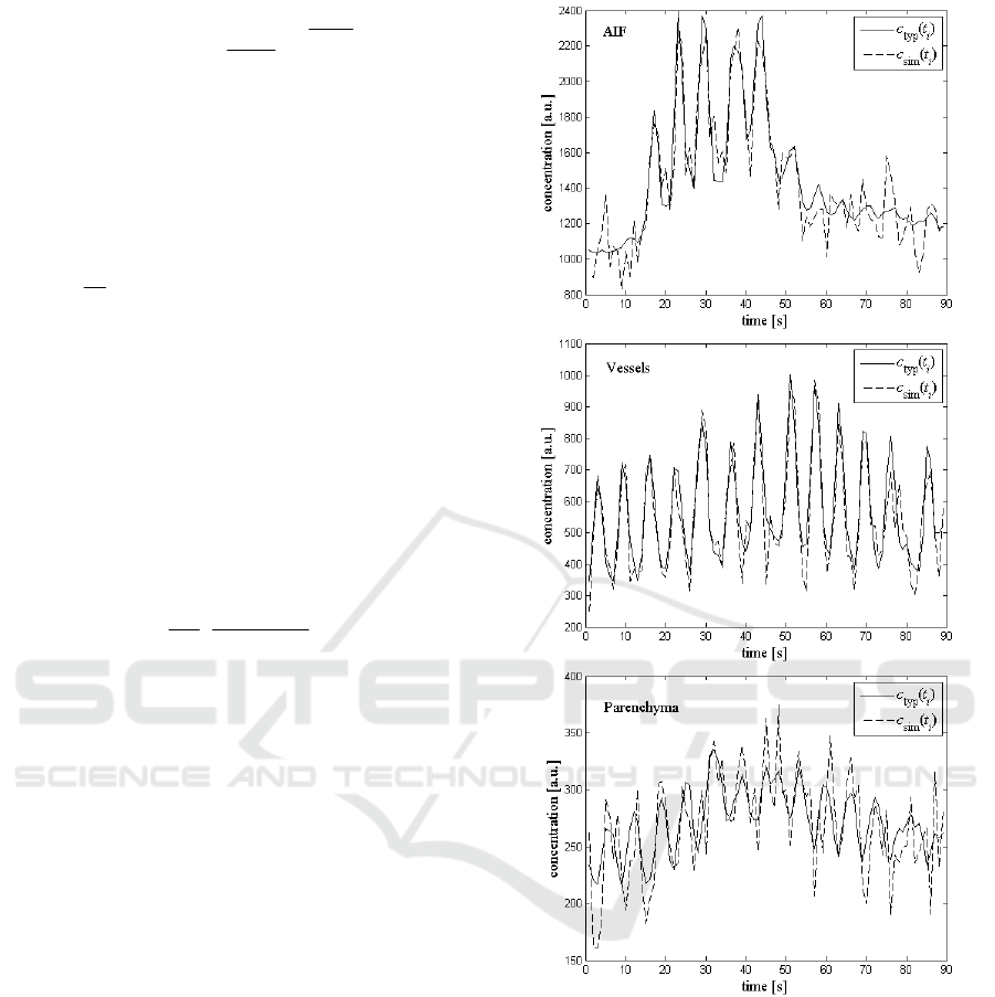
Figure 2 shows the c

typ

) and an example of a

sim

) for AIF, vessels and parenchyma.

The peaks and valleys (figure 2) are

characteristic for pCT lung results. They are caused

by the patient's breathing during the examination. In

further analysis we consider the peaks which

correspond to the phase of inspiration. The peaks

were detected using the function findpeaks

(Mathworks Matlab R2010a). Only the first passage

of tracer was modelled.

The following functions were chosen to be

compared:

 gamma-variate function;



010321

,,,,

ettvttvvvV





(3)

 Gauss function;



1321

,,,

egtgggG





(4)

 Rayleigh;

Proposal of New Tracer Concentration Model in Lung PCT Study - Comparison with Commonly Used Gamma-variate Model

135



1021

,,,

rttrrR











(5)

where v

, v

, g

, r

are regression

function parameters; t

is arrival time of contrast

agent, determined empirically.

The values of model parameters v = [v

, v

], g

= [g

, g

] and r = [r

, r

] were calculated

according to the objective function:

  



OFppp

tctc

minarg,..,,

min,

mod











(6)

where N is number of time points, p is the parameter

vector equal to v, g and r for the gamma-variate, the

Gauss and the Rayleigh model functions c

mod

,p),

respectively.

The BV parameter is the relative blood volume in

the considered ROI. It is defined as follows

(Calamante et al., 1999):









dttc

AIF



(7)

where k

is the correction factor accounting for the

differences in the hematocrit of capillaries and large

vessels, ρ is the tissue density [g/cm3], and c(t) and

AIF

(t) are the concentration of contrast agent in ROI

and in AIF, respectively. In literature the values of

and ρ differ significantly (Chan and Siochi, 2011;

Cohen, 1966; Hopkins et al., 2007; Lilienfeld et al.,

1956; Pevsner et al., 2005; Praveenkumar et al.,

2011). In our research the precise values of k

and ρ

are not relevant. We assume k

/ρ = 1 for all the

considered types of tissue: AIF, vessels,

parenchyma.

Next, the models will be used to calculate the

blood volume BV defined by the equation 7, which

is the diagnostically important descriptor of lung

perfusion. Errors associated with measurements

propagate to the errors associated with model

parameters and in turn they propagate to errors of

perfusion parameter BV. The way of propagation

depends on the particular form of the regression

function. We will test different regression functions

to compare their built-in, inner potential to provide

accurate identification results. To get the aim we

will apply methodology and criteria of the error

propagation and of the sensitivity analysis.

There are two basic questions relating to the

Figure 2: Typical concentration-time curves c

typ

) and an

example of the simulated curve c

sim

) for AIF (upper),

vessels (middle) and parenchyma (lower).

identification of model parameters. Is the model

identifiable, i.e. whether there is a unique solution in

form of model parameters? Whether the parameters

can be designated on the basis of the measurements

with a satisfactory accuracy?

It is important to obtain unique estimates of all

model parameters. This problem is considered as

theoretical or a priori identifiability. Sometime a

model is theoretically identifiable, but process of

parameters estimation may produce such large errors

that occurs a loss of practical or a posteriori

BIOSIGNALS 2017 - 10th International Conference on Bio-inspired Systems and Signal Processing

136

identifiability.

Process of parameters estimation requires finding

minimum of objective function OF in the parameter

space. Dimension of the parameter space is equal to

the number of model parameters n

≤N, N is number

of measurements:

  



OFppp

tyty

minarg,..,,

min,

modmeas











(8)

where y

meas

) is a set of measurements collected in

N time points t

and y

mod

(p,t

) is a model function

that depend on parameter vector p.

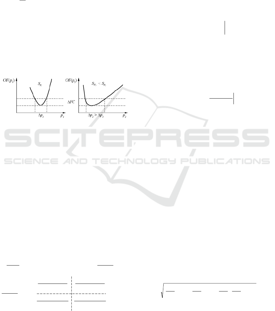
Let us analyse sensitivity S

of OF(p) with

respect to estimated parameters – for large and for

small sensitivity value. Assume that the resolution of

the OF measurement is OF, see Figure 3.

Figure 3: Dependence between the shape of OF and the

attainable accuracy for ∆p

and ∆p

> ∆p

for two model

parameters p

and p

and for the same measurement

resolution OF.

The larger sensitivity S

the smaller error p.

Therefore, for the same measurement resolution OF,

the attainable accuracy p differs depending on the

particular sensitivity function. The sensitivities are

dependent on the properties of the regression

function. Choice of the regression function of

desired properties is the aim of our investigation.

The relationship between sensitivity and error

one can present in an analytical form:

  





iiii

ttttOF ,,

modmeas

pyypyy 

(9)

where i = 1,...,N and p = [p

, p

,...,p

Differentiating OF with respect to the parameter

vector we obtain:

  

Nxn























),(),(

mod

1mod

mod

modmeas

pypy

pyy

(10)

S is the sensitivity matrix. Searching for error of

parameter estimates involves the searching for

variance-covariance matrix of the estimates. Under

simplifying assumptions (y

mod

(p,t

) is approximated

to a linear factor of Taylor series, the disturbances

are uncorrelated, the expected value of the

disturbances is zero, and covariance is constant and

equal to σ

) the variance-covariance matrix P in the

vicinity of the minimum of OF, takes the form of

(Cobelli et al., 2002; Enderle et al., 2000;

Semmelow, 2005):







minarg







SSPP

opt

xnn

opt



(11)

The matrix P is symmetric, as the variances are pair

wise symmetric. The sensitivity matrix S elements

are the sensitivities of the model output to changes

in particular parameters. The entries of the matrix P

are:

0)(det

21T2

)(det

)(adj

)(







SSP



xnn

(12)

When the matrix becomes singular: det(S

S)→0,

their entries are large and, therefore, associated error

estimates are large.

Even if structural identifiability of the model has

been previously confirmed, it may happen that the

matrix S

S is close to singular. Inversing such

matrix S

S cause very large entries of the matrix P,

which means a very large errors of parameter

estimates. Thus, the matrix S

S must be non-singular

and the sensitivity S large. Both, the sensitivity S

and the matrix S

S depend on the form of regression

function y

mod

. Choice of the regression function of

desired properties (large S and not singular, or not

close to singular, the matrix S

S) is the aim of our

investigation.

We assumed that model function is better than

the others if it gives lower objective function OF and

lower uncertainty ∆BV values. The smaller value of

OF, the better the function fit. According to the error

propagation rule, the smaller error pi of regression

function parameters the smaller ∆BV uncertainty of

BV. For example, when regression function depends

on two parameters p

and p

, then the uncertainty

∆BV is defined as follows (Ku, 1966):

BV 































































(13)

where Δp

, Δp

are parameters p

and p

estimation

errors, Δp

is estimated covariance of p

and p

In literature it is presented opinion that the first

passage of tracer is asymmetrical, i.e. the rising and

Proposal of New Tracer Concentration Model in Lung PCT Study - Comparison with Commonly Used Gamma-variate Model

137

falling edges are not equally sloped (Lampaskis et

al., 2009; Thompson et al., 1964). In order to

examine symmetry between rising and falling edge

of concentration-time measurements in pCT lung

study, the edges were approximated by linear

function in the range of linear edge course. The

slope angles



and 

were calculated. The

asymmetry coefficient

 was defined as follows:

%100













(14)

3 RESULTS

To compare the different regression functions 100

simulation runs were performed. For each simulation

run the value of objective function OF was

calculated for all compared regression functions.

Then, for each regression function the mean value of

the objective function was calculated. The results

obtained for AIF, vessels and parenchyma are

presented in table 1 - different regression functions

show different ability to fit measurements. Table 2

presents the mean BV and BV calculated according

to the error propagation rule, with respect to all

model parameters, for simulated data.

The value of BV, for AIF region and for all

regression functions, is known a priori and equal to

100, see table 2 and 4. It results from the equation 7:

the integrals in numerator and denominator of are

equal, so their quotient is equal to 1 and k

/ρ = 1. In

literature the BV is given in [ml/100g] therefore

equation 7 is multiplied by 100.

Table 1: Mean values of objective function for gamma-

variate, Gauss and Rayleigh functions in all regions

calculated for simulated data.

gamma-variate Gauss Rayleigh

AIF 9258 9198 9201

vessels 808 680 1218

parenchyma 193 186 230

Table 3 shows mean OF calculated for the actual

measurements taken from 5 subjects. Table 4 shows

example results of BV and ∆BV for a certain patient

calculated based on actual data.

Tables 5 shows rising and falling edge slope

angles



and 

, their differences and asymmetry

coefficients

, separately for each of 5 subjects.

Table 6 shows mean values of rising and falling

edge slope angles



and 

, their standard

deviations ∆



and ∆

, differences between mean

values of



and 

and asymmetry coefficients .

Table 2: Mean BV parameters; their uncertainties ±∆BV

and CV calculated for simulated data, taking into account

errors p

of regression functions parameters p

BV [ml/100g]

±ΔBV [ml/100g]

CV [%]

gamma-variate Gauss Rayleigh

AIF

100

±0,2626

0,2626

100

±0,0760

0,0760

100

±0,2447

0,2447

vessels

19,1400

±61,5489

321,5700

19,9783

±0,0058

0,0290

21,0502

±0,0333

0,1582

parenchyma

6,1652

±0,0680

1,1030

6,2627

±0,0004

0,0064

5,6497

±0,0051

0,0903

Table 3: Mean values of objective function for gamma-

variate, Gauss and Rayleigh functions in all regions

calculated for 5 subjects, based on actual data.

gamma-variate Gauss Rayleigh

AIF 9411 7791 9129

vessels 853 706 1401

paren. 136 130 139

Table 4: Example results of BV parameter; its uncertainty

±∆BV and CV calculated for single subject (female, 63

years old), taking into account errors p

of regression

functions parameters p

, based on actual data.

BV [ml/100g]

±ΔBV [ml/100g]

CV [%]

gamma-variate Gauss Rayleigh

AIF 100

±0,1170

0,1170

100

±0,0311

0,0311

100

±0,2505

0,2505

vessels 10,3512

±20,2722

195,8440

8,5467

±0,0037

0,0433

11,0668

±0,0158

0,1428

parenchyma 8,4072

±0,0084

0,0999

8,1724

±0,0004

0,0049

8,3620

±0,0075

0,0897

Table 5: Rising and falling edge slope angles 

and 

their differences and asymmetry coefficients  calculated

for 5 subjects, based on actual data.



R []



F [] |R|-|F| []



[%]

AIF 88,24 -88,70 -0,46 -0,52

vessels 87,26 -86,04 1,22 1,40

parenchyma 77,64 -75,41 2,23 2,87

AIF 86,71 -87,94 -1,23 -1,42

vessels 85,53 -84,56 0,97 1,13

parenchyma 74,86 -69,65 5,21 6,96

BIOSIGNALS 2017 - 10th International Conference on Bio-inspired Systems and Signal Processing

138

Table 5: Rising and falling edge slope angles



and



their differences and asymmetry coefficients  calculate

for 5 subjects, based on actual data (cont.).

AIF 89,59 -89,02 0,57 0,64

vessels 85,37 -87,16 -1,79 -2,10

parenchyma 71,83 -73,00 -1,17 -2,57

AIF 88,41 -88,15 0,26 0,29

vessels 84,42 -75,40 9,02 10,69

parenchyma 79,22 -66,50 12,72 16,06

AIF 88,91 -88,96 -0,05 -0,06

vessels 86,40 -86,30 0,10 0,12

parenchyma 64,73 -66,50 -1,77 -2,73

Table 6: Mean values of rising and falling edge slope

angles 

and 

, their standard deviations 

and 

differences and asymmetry coefficients  calculated for 5

subjects, based on actual data.

R []

±ΔR []

F []

±ΔF[]

|R|-

|F| []



[%]

AIF 88,37

±1,07

-88,55

±0,49

-0,18

0,21

vessels 85,80

±1,08

-83,89

±4,84

1,90 2,22

parenchyma 73,66

±5,73

-70,21

±3,96

3,44 4,68

4 DISCUSSION

Our aim is to determine which function best

approximates the first passage of tracer in pCT lung

studies. Fitting results, presented in table 1, show

different quality of fit for different regression

functions. Taking into account OF values, the Gauss

function proved to be the best in all considered

regions - AIF, vessels and parenchyma. Similar

conclusions can be drawn on the basis of uncertainty

analysis, see table 2. It is worth mentioning, that the

most frequently used gamma-variate function

produced noticeably higher BV than the Gauss and

the Rayleigh functions.

Simulated data analysis demonstrated the

advantage of the Gauss function over the other ones.

In order to confirm the simulation results, actual

measurements analysis was performed. The results,

presented in table 3, show that OF in all regions are

the lowest for the Gauss function. The Gauss

function best approximates the first passage of tracer

in AIF, blood vessels and parenchyma. Also, the

Gauss function produces the lowest uncertainty BV,

which means that the impact of model parameters

error on BV is the smallest.

It is widely accepted that the first passage of

tracer is asymmetrical, i.e. the rising and falling

edges are not equally sloped (Lampaskis et al., 2009;

Thompson et al., 1964). Considering this, regression

function that best approximates the first passage of

tracer should also be asymmetrical. However, it was

proved (table 1 and table 3) that the Gauss function,

which is symmetrical, best approximates the first

passage of tracer. The rising and falling edges of

concentration-time curves were approximated by the

linear function and slope angles were calculated.

Rising and falling edge slope angles, their

differences and asymmetry coefficients calculated

for 5 subjects are presented in table 5. Furthermore,

the mean values of slope angles, their standard

deviations, differences and asymmetry coefficients

were calculated and presented in table 6. Differences

between slope angles are insignificant and the

differences between mean values of rising and

falling edge slope angles, presented in table 6, are

negligible. Therefore, it can be assumed that rising

and falling edges of actual measurements are

symmetrical (very close to symmetrical). For that

reason, the Gauss function proved to be best

approximation of the first passage of tracer in pCT

lung studies.

5 CONCLUSIONS

This paper presents a comparative analysis of three

regression functions in three regions (AIF, blood

vessels and parenchyma) in pCT lung tests.

Considering results of simulated data analysis, the

Gauss function showed a clear advantage over the

others. Results of actual measurements analysis

confirmed that the Gauss function produce the most

accurate approximations of the first passage of

tracer. It was showed that contrary to the widely

accepted practice, the differences between rising and

falling edge slope angles of concentration-time

curves are inconsiderable. Therefore, one can

assume that rising and falling edges are symmetrical.

Negligible asymmetry of measurements justifies

why the Gauss function best approximates the first

passage of tracer in pCT lung studies.

ACKNOWLEDGEMENTS

This work was supported by funds of Faculty of

Electronics, Telecommunications and Informatics,

Gdańsk University of Technology.

Proposal of New Tracer Concentration Model in Lung PCT Study - Comparison with Commonly Used Gamma-variate Model

139

REFERENCES

Balthazar, E. (2011). CT Contrast Enhancement of the

Pancreas: Patterns of Enhancement, Pitfalls and

Clinical Implications. Pancreatology, 11(6), pp.585-

587.

Balvay, D., Ponvianne, Y., Claudon, M. and Cuenod, C.

(2008). Arterial input function: Relevance of eleven

analytical models in DCE-MRI studies. In:

Proceedings of 5th IEEE International Symposium on

Biomedical Imaging. Paris: IEEE.

Blomley, M. and Dawson, P. (1997). Bolus dynamics:

theoretical and experimental aspects. The British

Journal of Radiology, 70(832), pp.351-359.

Browarczyk, M., Kalicka, R. and Lipiński, S. (2015).

Lung Perfusion Parameters in the Diagnosis of

Diabetic Pulmonary Microangiopathy. In: I. Lacković

and D. Vasic, ed., 6th European Conference of the

International Federation for Medical and Biological

Engineering, 1st ed. Dubrovnik: Springer International

Publishing, pp.444-447.

Calamante, F., Thomas, D., Pell, G., Wiersma, J. and

Turner, R. (1999). Measuring Cerebral Blood Flow

Using Magnetic Resonance Imaging Techniques.

Journal of Cerebral Blood Flow & Metabolism,

pp.701-735.

Cao, Y. (2011). The Promise of Dynamic Contrast-

Enhanced Imaging in Radiation Therapy. Seminars in

Radiation Oncology, 21(2), pp.147-156.

Chen, M. and Siochi, R. (2011). Feasibility of using

respiratory correlated mega voltage cone beam

computed tomography to measure tumor motion.

Journal of Applied Clinical Medical Physics, 12(2),

p.3473.

Cobelli, C., Foster, D. and Toffolo, G. (2002). Tracer

kinetics in biomedical research. New York: Kluwer

Academic.

Cohen, M. (1966). The Organization of Clinical

Dosimetry: I. the four stages of clinical dosimetry.

Acta Radiologica: Therapy, Physics, Biology, 4(3),

pp.233-256.

Enderle, J., Blanchard, S. and Bronzino, J. (2000).

Introduction to biomedical engineering. San Diego:

Academic Press.

Hopkins, S., Henderson, A., Levin, D., Yamada, K., Arai,

T., Buxton, R. and Prisk, G. (2007). Vertical gradients

in regional lung density and perfusion in the supine

human lung: the Slinky effect. Journal of Applied

Physiology, 103(1), pp.240-248.

Jackson, A. (2004). Analysis of dynamic contrast

enhanced MRI. The British Journal of Radiology,

77(suppl_2), pp.S154-S166.

Kalicka, R. and Pietrenko-Dąbrowska, A. (2006).

Parametric Modeling of DSC-MRI Data with

Stochastic Filtration and Optimal Input Design Versus

Non-Parametric Modeling. Annals of Biomedical

Engineering, 35(3), pp.453-464.

Kalicka, R., Browarczyk, M. and Lipiński, S. (2015).

Usefulness of chest perfusion computed tomography

in the diagnosis of diabetic pulmonary

microangiopathy. Biocybernetics and Biomedical

Engineering, 35(1), pp.68-73.

Ku, H. (1966). Notes on the use of propagation of error

formulas. Journal of Research of the National Bureau

of Standards, Section C: Engineering and

Instrumentation, 70C(4), p.263.

Lampaskis, M., Strouthos, C. and Averkiou, M. (2009).

Application of tracer dilution models for the

quantification of perfusion with contrast enhanced

ultrasound imaging. In: Proceedings of 14th European

Symposium on Ultrasound Contrast Imaging.

Rotterdam.

Lilienfield, L., Kovach, R., Marks, P., Hershenson, L.,

Rodnan, G., Ebaugh, F. and Freis, E. (1956). THE

HEMATOCRIT OF THE LESSER CIRCULATION

IN MAN 12. Journal of Clinical Investigation, 35(12),

pp.1385-1392.

Mírka, H., Ferda, J., Baxa, J., Třeška, V., Liška, V.,

Schmidt, B. and Flohr, T. (2010). Perfusion CT of the

liver. Czech Radiology, 64(4), pp.281-289.

Nakano, S., Gibo, J., Fukushima, Y., Kaira, K., Sunaga,

N., Taketomi-Takahashi, A., Tsushima, Y. and Mori,

M. (2013). Perfusion Evaluation of Lung Cancer.

Journal of Thoracic Imaging, 28(4), pp.253-262.

Ng, Q. and Goh, V. (2010). Angiogenesis in Non-small

Cell Lung Cancer. Journal of Thoracic Imaging,

25(2), pp.142-150.

Pevsner, A., Nehmeh, S., Humm, J., Mageras, G. and Erdi,

Y. (2005). Effect of motion on tracer activity

determination in CT attenuation corrected PET images:

A lung phantom study. Med. Phys., 32(7), p.2358.

Praveenkumar, R., Augustine, A. and Santhosh, K. (2011).

Estimation of inhomogenity correction factors for a

Co-60 beam using Monte Carlo simulation. Journal of

Cancer Research and Therapeutics, 7(3), p.308.

Sauter, A., Feldmann, S., Spira, D., Schulze, M., Klotz, E.,

Vogel, W., Claussen, C. and Horger, M. (2012).

Assessment of Splenic Perfusion in Patients with

Malignant Hematologic Diseases and Spleen

Involvement, Liver Cirrhosis and Controls Using

Volume Perfusion CT (VPCT). Academic Radiology,

19(5), pp.579-587.

Semmlow, J. (2005). Circuits, signals, and systems for

bioengineers. Oxford: Academic.

Srikanchana, R., Thomasson, D., Choyke, P. and Dwyer,

A. (2004). A comparison of pharmacokinetic models

of dynamic contrast enhanced MRI. In: Proc. IEEE

Symp. Computer-Based Med. Syst.. Bethesda: IEEE,

pp.361-366.

Thompson, H., Starmer, C., Whalen, R. and Mcintosh, H.

(1964). Indicator Transit Time Considered as a Gamma

Variate. Circulation Research, 14(6), pp.502-515.

Wintermark, M., Sincic, R., Sridhar, D. and Chien, J.

(2008). Cerebral perfusion CT: Technique and clinical

applications. Journal of Neuroradiology, 35(5),

pp.253-260.

Zhao, H., Gong, J., Wang, Y., Zhang, Z. and Qin, P.

(2010). Renal hemodynamic changes with aging: a

preliminary study using CT perfusion in the healthy

elderly.

Clinical Imaging, 34(4), pp.247-250.

BIOSIGNALS 2017 - 10th International Conference on Bio-inspired Systems and Signal Processing

140