Optimizing Spare Battery Allocation in an Electric Vehicle Battery

Swapping System

Michael Dreyfuss and Yahel Giat

Department of Industrial Engineering, Jerusalem College of Technology, HaVaad HaLeumi 21, Jerusalem, Israel

Keywords:

Battery Swapping, Electric Vehicle, Exchangeable Item Repair System, Window Fill Rate, Spare Allocation

Problem

Abstract:

Electric vehicle battery swapping stations are suggested as an alternative to vehicle owners recharging their

batteries themselves. To maximize the network’s performance spare batteries must be optimally allocated in

these stations. In this paper, we consider the battery allocation problem where the criterion for optimality is

the window ﬁll rate, i.e., the probability that a customer that enters the swapping station will exit it within a

certain time window. This time is set as the customer’s tolerable wait in the swapping station. In our derivation

of the window ﬁll rate formulae, we differ from previous research in that we assume that the swapping time

itself is not negligible. We numerically analyse the battery allocation problem for a hypothetical countrywide

application in Israel and demonstrate the importance of estimating correctly customers’ tolerable wait, the

value of reducing battery swapping time and the unique features of the optimal battery allocation.

1 INTRODUCTION

Electric vehicles’ batteries need to be recharged fre-

quently with inconveniently long recharging time.

The US-based corporation Better Place suggested to

overcome this problem by separating battery owner-

ship from the vehicle’s ownership so that customers

purchase the vehicle from the auto-maker and lease

battery services from a third party (“the ﬁrm”). The

ﬁrm will construct a network of battery swapping sta-

tions in which car owners replace their depleted bat-

teries for charged ones from the station’s stock. Sep-

arately, the depleted batteries are recharged and put

back in the stock to be given to future customers. To

improve the network’s performance, the ﬁrm may de-

cide to place spare batteries in each station. There-

fore, given a total budget of spare batteries, the ﬁrm

must decide how to allocate the spare batteries among

the battery swapping stations with the goal of opti-

mizing a predetermined service measure.

The service measure that we consider in this paper

is a generalization of the ﬁll rate. With the ﬁll rate, the

ﬁrm will allocate batteries to maximize the fraction

of customers who are served upon arrival. In reality,

however, the ﬁll rate is rarely an accurate proxy for

the ﬁrm’s costs. For example, if the battery provider is

obliged by contractual commitment to provide service

within a certain time then it does not need to have a

battery ready for the customer immediately when she

arrives. From the customers’ standpoint, too, there is

a certain tolerable or acceptable period of wait, which

may depend on their level of patience or expectation.

If a customer entering the station expects being served

within the ten minutes it would take to ﬁll a tank of a

conventional car, then the ﬁrm experiences reputation

and contractual losses only if the customer waits more

than ten minutes. Thus, the ﬁrm’s objective should be

to maximize the window ﬁll rate, i.e., the probability

that a customer is served within the tolerable wait.

To address this problem, we use research in the

ﬁeld of exchangeable-item repair systems. Customers

arrive to these systems with a failed item and ex-

change it for an operable item in a manner similar

to the battery swapping scheme. Furthermore, since

battery charging docks are relatively inexpensive, one

may assume that there are ample servers in each lo-

cation so that each location can be modelled as an

M/G/∞ queue. (Dreyfuss and Giat, 2016) develop an

algorithm for ﬁnding a near-optimal solution in such

multi-location systems assuming that the item’s as-

sembly and disassembly times are negligible. This

assumption is clearly unrealistic for the battery swap-

ping problem since battery removal and installation

times are signiﬁcant compared to the customer’s tol-

erable wait.

In this paper, we develop the window ﬁll rate for-

38

Dreyfuss M. and Giat Y.

Optimizing Spare Battery Allocation in an Electric Vehicle Battery Swapping System.

DOI: 10.5220/0006115000380046

In Proceedings of the 6th International Conference on Operations Research and Enterprise Systems (ICORES 2017), pages 38-46

ISBN: 978-989-758-218-9

Copyright

c

mula for the case of positive item assembly and disas-

sembly times and show that a ∆ increase in the assem-

bly and disassembly time is equivalent to a ∆ decrease

in the tolerable wait. Using this ﬁnding we apply the

(Dreyfuss and Giat, 2016) algorithm to ﬁnd a solution

to the battery swapping problem, i.e., how to allocate

spare batteries in the network, and make the following

contributions.

We estimate the battery allocation problem of the

Better Place corporation if it had succeeded going

widespread in Israel and derive the optimal solution

for different service criteria. This example provides

valuable insight into the critical importance of assess-

ing correctly the tolerable wait time and the signiﬁ-

cant losses that the ﬁrm incurs if it neglects to do so.

Second, we estimate the savings attained by reducing

battery swapping time. Third, we show how customer

arrival rate creates two classes of battery exchange

stations and therefore managers should develop two

different policies with respect to their service time to

customers. Although the Better Place adventure has

ended with bankruptcy in 2013, the battery swapping

idea is either applied or considered by other compa-

nies (e.g. XJ Group Corporation in Qingdao, Tesla

in California and Gogoro in Taipei). The model pre-

sented in this paper, therefore, may yet be applied in

real-life large-scale situations.

2 LITERATURE REVIEW

Electric vehicles are considered an environmentally-

friendly alternative to internal combustion engine cars

and are projected to eventually replace these fuel-

burning cars (Dijk et al., 2013). Drivers, however,

are still wary of these vehicles and therefore, many

governments provide substantial tax incentives to en-

courage their widespread adoption. Notable examples

are West European countries, the United States, China

and Japan (Zhou et al., 2015). Despite these efforts,

many drivers are wary of purchasing these cars and

most governments adoption goals have not been met

(Coffman et al., 2016). The major customer concern

is the “range anxiety”, namely, the fact that batteries

have limited range and their recharging time is very

long compared to internal combustion engine cars.

An innovative idea to overcome these issues was in-

troduced by the US-based company Better Place who

proposed to separate the vehicle ownership from the

battery ownership. In lieu of owning the battery, car

owners will purchase battery services from a ﬁrm that

will establish a network of battery swapping stations.

Researcher are examining many aspects of this propo-

sition such as the station design, the battery removal

and installation times, the required number of spare

batteries and the network layout and managing the

loads on the power grid (Mak et al., 2013; Yang and

Sun, 2015; Sarker et al., 2015). We contribute to

this research by solving the spare battery allocation

problem and demonstrating a large-scale application

of this problem.

The assumption that customers will tolerate a cer-

tain wait is at the core of this paper, which lies at the

intersection of inventory and customer service mod-

els. While the concept of a tolerable wait is hardly

ever considered in inventory models, it is quite com-

mon in the service industry and is associate with

numerous terms such as “expectation” (Durrande-

Moreau, 1999), “reasonable duration” (Katz et al.,

1991), “maximal tolerable wait” (Smidts and Pruyn,

1999) and “wait acceptability” (Demoulin and Dje-

lassi, 2013). From a service-oriented approach, the

customer’s attitude to wait is mainly subjective and

has cognitive and affective aspects (Demoulin and

Djelassi, 2013). From a logistics point of view this

wait is more objective and usually stated in the service

contract. Indeed, researchers have observed that most

inventory models fail “to capture the time-based as-

pects of service agreements as they are actually writ-

ten” (Caggiano et al., 2009, p.744). Our paper ﬁlls

this void by incorporating the tolerable wait into the

optimization criterion.

Our battery swapping network may be modelled

as an exchangeable-item repair system (Avci et al.,

2014). These inventory systems have been investi-

gated by researchers in different contexts (Basten and

van Houtum, 2014). A common performance mea-

sure for such systems is the ﬁll rate, which measures

the fraction of customers who are served upon ar-

rival (Shtub and Simon, 1994; Caggiano et al., 2007).

These papers, however, do not develop explicit for-

mulas for the window ﬁll rate but use numerical tech-

niques. In contrast, (Berg and Posner, 1990) develop

a formula for the window ﬁll rate in a single loca-

tion when item assembly and disassembly is zero, and

(Dreyfuss and Giat, 2016) ﬁnd that the window ﬁll

rate is generally S-shaped with number spares in the

location and exploit this property to develop an efﬁ-

cient near-optimal algorithm for ﬁnding the optimal

spare allocation. We extend these papers by consid-

ering the case of positive assembly and disassembly

times.

3 THE MODEL

Customers arrive with a depleted battery to a battery

swapping network that comprises L stations. Upon ar-

Optimizing Spare Battery Allocation in an Electric Vehicle Battery Swapping System

39

rival, the battery is removed and placed in a charging

dock and once it is fully recharged it is added to the

station’s stock. To reduce customer waiting time, the

network keeps a number of spare batteries, so that if

there is a spare battery available on stock it is installed

in the client’s vehicle in exchange of the depleted bat-

tery that she had brought. Customers are served ac-

cording to a ﬁrst-come, ﬁrst-serve policy and leave

the swapping station once their battery is replaced.

For each station l, l = 1, ...,L, we assume that cus-

tomer arrival rate follows an independent Poisson pro-

cess with parameter λ

l

(see (Avci et al., 2014) for

a justiﬁcation of this assumption). We assume that

there are ample charging docks in each station and

that charging time at each dock is i.i.d. The combina-

tion of these two assumptions is that once the battery

is removed from the vehicle, charging commences

immediately and that recharging times are indepen-

dent. Let R

l

(t) denote the cumulative probability of a

battery to be recharged by time t and let r

l

denote the

mean recharging time. Battery removal and battery

installation times are t

1

and t

2

, respectively. The bat-

tery swapping time, t

1

+t

2

, is assumed to be no more

than the tolerable wait.

3.1 Single Station

Consider a random customer, Jane, that arrives at time

s to station l that was allocated b spares. The non-

stationary window ﬁll rate, F

NS

l

(s,t, b) is the proba-

bility that Jane will exit the station by time s +t. This

happens if and only if by date s+t −t

2

Jane is at the

head of the queue and there is at least one charged bat-

tery available at the station’s stock. By “head of the

queue” we mean that all the customers who arrived

before Jane (“Pre-Jane customers”) have either exited

the station or are in the process of installing batteries

in their vehicles. We can ensure this by verifying a

supply and demand equation for recharged batteries.

On the supply side, we consider the initial number of

spare batteries in the station, b, plus all the batteries

whose recharging was completed during the time seg-

ment [0,s+t−t

2

]. On the demand side we consider the

number of Pre-Jane customer plus Jane herself. Let:

• N

1

denote the number of batteries brought by Pre-

Jane customers who were recharged before s+t−

t

2

.

• N

2

denote the number of batteries brought by Pre-

Jane customers who were recharged after s+t−t

2

.

• N

3

denote the number of batteries brought by cus-

tomers who arrived after Jane (“Post-Jane cus-

tomers”) and were recharged before s+t−t

2

.

• Z denote a Binary variable that is equal to one if

Jane’s battery is recharged by s+t −t

2

and zero

otherwise.

The probability that Jane will exit the station by

s + t is the probability that the supply is greater than

the demand as follows

F

NS

l

(s,t,b) = Pr[Supply ≥ Demand]

= Pr[b+N

1

+Z+N

3

≥ N

1

+N

2

+1]

= Pr[b + Z + N

3

≥ N

2

+ 1] (1)

Since the battery brought by Jane begins recharg-

ing at s+t

1

, the probability for Z = 1 is the probability

that a battery completes recharging during the inter-

val [s + t

1

,s + t − t

2

], which is equal to R

l

(t −t

1

−t

2

).

Therefore, we can condition on the value of Z and

rewrite (1) as

F

NS

l

(s,t,b) = R

l

(t−t

1

−t

2

)Pr[b+1+N

3

≥ N

2

+1]

+



1 − R

l

(t−t

1

−t

2

)



Pr[b+N

3

≥ N

2

+1]

= Pr[N

2

−N

3

≤b−1] + R

l

(

ˆ

t)Pr[N

2

−N

3

=b], (2)

where

ˆ

t := t −t

1

−t

2

.

Our assumption that batteries arrive according to

a Poisson process and the ample server assumption

guarantee that N

2

and N

3

are independent Poisson ran-

dom variables that are also independent of Z. Recall,

N

2

is the number of batteries who arrived between

[0,s] and were not repaired by s + t − t

2

. Of these

customers, consider a customer that arrives during

the time interval [u, u + du] in [0, s]. Due to the con-

ditional uniform distribution property of the Poisson

process, the probability for this is du/s (Ross, 1981,

Chapter 3.5). This customer’s battery is removed

and begins to be recharged at u + t

1

. The probabil-

ity that recharging is completed only after s + t −t

2

is

1 − R

l



s +t − t

2

− (u +t

1

)



. Thus,

N

2

∼ Poisson



λ

l

s

Z

u=0



1−R

l

(s+t−t

2

−u−t

1

)



du

s



∼ Poisson



λ

l

s+

ˆ

t

Z

u=

ˆ

t



1−R

l

(u)



du



. (3)

To derive the distribution of N

3

we consider the

customers who arrived between [s,s + t − t

2

] and

whose batteries were recharged by s + t−t

2

. Of these

customers, consider a customer that arrives during the

time interval [u,u + du]. The probability for this is

du/(t −t

2

). This customer’s battery is removed and

begins to be recharged at u + t

1

. The probability

that recharging is completed by s +t − t

2

is, therefore

ICORES 2017 - 6th International Conference on Operations Research and Enterprise Systems

40

R

l



s +t − t

2

− (u +t

1

)



. Thus,

N

3

∼ Poisson



λ

l

(t−t

2

)

s+t−t

2

Z

u=s

R

l

(s+t−t

2

−u−t

1

)

du

t−t

2

∼ Poisson



λ

l

ˆ

t

Z

u=−t

1

R

l

(u)du = λ

l

ˆ

t

Z

u=0

R

l

(u)du



. (4)

The stationary window ﬁll rate is obtained by tak-

ing the limit of s in (3) to inﬁnity, which results with

the following proposition:

Proposition 1. The stationary window ﬁll rate for

station l with b spares is given by

F

l

(t,b) = Pr[N ≤ b − 1] + R

l

(

ˆ

t)Pr[N = b] (5)

where N :=N

2

−N

3

and where N

3

is deﬁned in (4) and

N

2

∼Poisson



λ

l

∞

R

u=

ˆ

t

(1−R

l

(u))du



.

3.2 The Network

Let

~

b = (b

1

,...,b

L

) be a network battery allocation

and let λ :=

∑

λ

l

denote the (total) arrival rate to the

network. The network’s window ﬁll rate, F(t,

~

b), is

the weighted average of the local window ﬁll rates.

Therefore, given a budget of B spare batteries, the bat-

tery allocation problem is:

max

~

b≥0

F(t,

~

b) :=

L

∑

l=1

λ

l

λ

F

l

(t,b

l

) s.t.

L

∑

l=1

b

l

= B. (6)

Since the window ﬁll rate depends only on

ˆ

t =

t −t

1

− t

2

we can instead assume that the battery re-

moval and installment times are zero and use the ad-

justed tolerable wait,

ˆ

t, in lieu of the true tolerable

wait t. The implication of this observation is that

we can use the results of (Dreyfuss and Giat, 2016)

who assume zero swapping time. In the remainder

of this section, we apply the results of (Dreyfuss and

Giat, 2016) to our model with positive swapping time.

We state only the results that are necessary for under-

standing the battery allocation application.

6

-

0.25

0.5

0.75

1

F

l

(t,b)

Number of Spare Batteries

b

.

F

l

(t,b)

tangent line

q

m

l

@

@I

tangent point

Figure 1: The window ﬁll rate for an S-shaped station.

Result 1: The Shape of the Window Fill Rate

F

l

(t,b) is strictly increasing in b. If t ≥ r

l

+t

1

+t

2

then

F

l

(t,b) is concave in b. Otherwise, F

l

(t,b) is either

concave in b or initially convex and then concave (S-

shaped) in b. The tangent point decreases with t and

increases with t

1

+t

2

.

Result 2: The Optimization Algorithm

By (6), the window ﬁll rate is a separable sum of

either concave or S-shaped functions. For each S-

shaped station we deﬁne the tangent point, m

l

, as

the ﬁrst integer such that



F

l

(t,m

l

) − F

l

(t,0)



/m

l

>

∆F

l

(t,m

l

), where ∆F

l

(t,b) is the ﬁrst difference of

F

l

(t,b) and is given by

∆F

l

(t,b):=F

l

(t,b+1)−F

l

(t,b)

=



1−R

l

(t)



Pr[N =b] + R

l

(t)Pr[N =b+1]. (7)

For concave stations we set the tangent point to zero.

For each station, let H

l

(t,b) denote the concave cov-

ering function of F

l

(t,b) in the following manner:

H

l

(t,b)=

(

F

l

(t,0)+

F

l

(t,m

l

)−F

l

(t,0)

m

l

b if 0 ≤b ≤m

l

−1

F

l

(t,b) if b ≥ m

l

.

That is, for any b smaller than the tangent point, we

replace F

l

(t,b) with the straight line connecting the

point



0,F

l

(t,0)



and the point



m

l

,F

l

(t,m

l

)



. By

construction, for all b ≥ 0,H

l

(t,b) is concave and

H

l

(t,b) ≥ F

l

(t,b). Finally, we deﬁne H(t,

~

b) as the

weighted sums of all the stations’ functions H

l

(t,b

l

)

similarly to (6).

Since H(t,

~

b) is a separable sum of concave func-

tions we can use a greedy algorithm to maximize it.

This algorithm will choose the “best for the buck” sta-

tion and since H

l

is initially linear, it will stay with

stay with this station until it has reached the station’s

tangent point. It then continues with the next best sta-

tion and so forth. Before switching to the next linear

slope it is possible that stations that have reached their

tangent will get additional spares (as long as their cur-

rent slope is steeper than the next best linear slope).

However, once a region begins receiving slopes in its

linear region, it will be the only one to receive spares

until it has reached its tangent point. Consequently,

the algorithms produces an allocation with properties

stated in the following result.

Result 3: The Optimal Allocation

~

b

H

satisﬁes one of the following two cases:

1. For every l = 1 ...L, either b

H

l

≥ m

l

or b

H

l

= 0 and

the optimal solution to (6),

~

b

F

=

~

b

H

.

Optimizing Spare Battery Allocation in an Electric Vehicle Battery Swapping System

41

2. There exists a single station, denoted by

ˆ

l such

that 0 < b

H

ˆ

l

< m

ˆ

l

. For every other station l 6=

ˆ

l,

either b

H

l

≥ m

l

or b

H

l

= 0. In this case:

(a) The optimal value of F is bounded above by

H(t,

~

b

H

).

(b) The distance from optimum is bounded by

λ

ˆ

l

λ



H

ˆ

l

(t,b

H

ˆ

l

) − F

ˆ

l

(t,b

H

ˆ

l

)



.

4 NUMERICAL APPLICATION

The US-based corporation Better Place was founded

in 2007 with the ambitious goal of a large-scale adop-

tion of fully electric cars. Since battery-related issues

are the greatest obstacle to achieving this goal, Better

Place developed a unique business model in which it

retained battery ownership. Customers were to pur-

chase the car absent the battery and Better Place was

to provide battery swapping and recharging services

and to assume all the battery-related risks (Dijk et al.,

2013).

Although Better Place has ﬁled for bankruptcy in

2013, its business model is still considered a promis-

ing solution to solving the battery problem in the elec-

tric car industry (Avci et al., 2014). Most of the cars

produced for Better Place’s customers were sold in

Israel, in which Better Place even completed the con-

struction of ﬁfty battery swapping stations before it

ﬁled for bankruptcy. The following section is a hy-

pothetical full scale application of the Better Place

model in a country with geographical and demograph-

ical characteristics similar to Israel.

Each of the three largest gas companies in Israel

operate approximately two hundred ﬁfty gas stations

and accordingly we assume that the battery service

ﬁrm (“the ﬁrm”) operates a network of two hundred

ﬁfty battery swapping stations distributed through-

out the country, with a total arrival of approximately

14,000 customers per hour. The population density

in Israel is such that the center region is the densest,

followed by the northern region. The south of Israel,

which constitutes more than half of Israel’s land area,

is sparsely populated. Therefore, the number of sta-

tions per customer in the south is higher than the num-

ber of stations in the center, reﬂecting the large geo-

graphical size that must be serviced. To model the

differences between the different stations in Israel, as

well as differences between small neighborhood sta-

tions and busy major stations we assume that the ar-

rival rates to the stations are equally spaced between

6.4 and 106 customers per hour.

An empty battery can be recharged to 50% of ca-

pacity within twenty minutes (Bullis, 2013). Since

there are many factors that affect recharging time we

assume that the recharging time is distributed nor-

mally with mean forty minutes and standard devia-

tion ten minutes. Battery swapping time, i.e., the bat-

tery removal and battery installation, is considerably

shorter than recharging time and with state-of-the-art

design, battery swapping can be done in less than

two minutes (Mak et al., 2013). Each station is as-

sumed to have ample battery rechargers since recharg-

ing docks are relatively inexpensive. Since the elec-

tric vehicle cars are poised as an alternative to the

traditional gasoline-fueled cars, we assume that the

tolerable wait for refueling is similar for both cars.

Anecdotal evidence suggests that a ten minute wait

for battery swapping is tolerated by customers. Fi-

nally, we use a baseline budget of nine thousand spare

batteries.

To summarize, the baseline parameters of the ex-

ample are: L = 250 stations; N = 9000 spare batteries;

λ

l

= 6+0.4 · l customers per hour, t

1

+t

2

= 2 minutes,

R

l

∼ Normal(40,10

2

) minutes and the optimization

criterion is the window ﬁll rate for a tolerable wait

t = 10 minutes(F10).

4.1 The Baseline Scenario

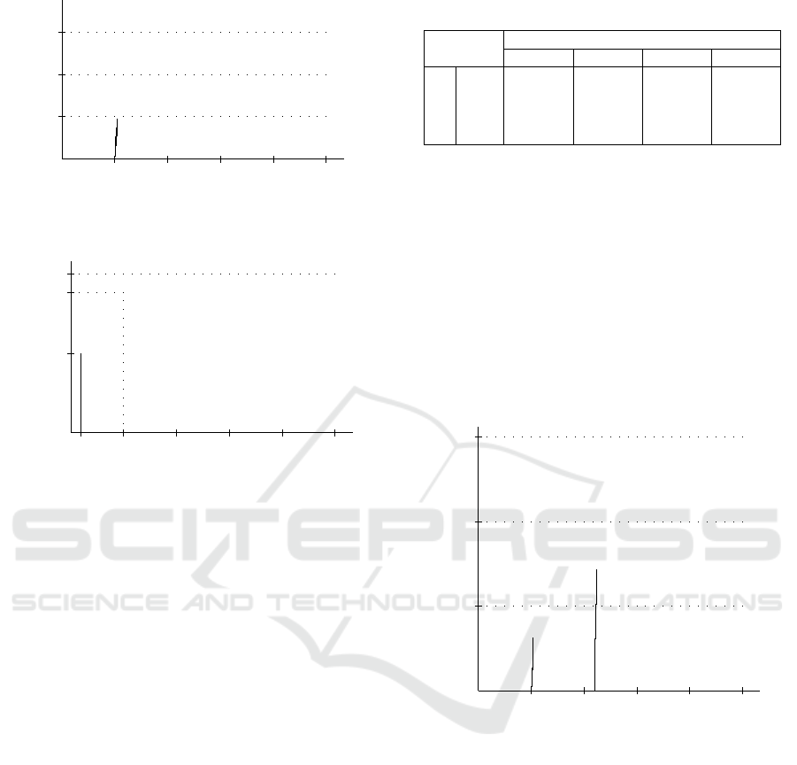
Figure 2 describes the near-optimal spare allocation

for the baseline case,

~

b

H

, and Figure 3 displays the

window ﬁll rate for the optimal allocation as a func-

tion of t, F(

~

b

H

,t). Recall, that the optimization algo-

rithm supplies spares to the station with the steepest

slope until it reaches its tangent point and only then

proceeds to the next station. The tangent line’s slope

and the tangent point are increasing with the arrival

rate and therefore the bigger the station index, the

greater the tangent point. The near-optimal alloca-

tion dictates that the 50 slowest-moving stations will

have no spares, whereas each of the busier stations

will receive at least its tangent point. Station 51 is the

exception; it has only two spares although its tangent

point is 19 (see case 1 of Result 3). This implies that

the solution F(

~

b

H

,10) = 88.5% is a lower bound that

it not necessarily optimal. However, the distance be-

tween the bounds is a mere 0.02% (see notes to Table

1).

The low arrival rate stations are not given any

spares and consequently, their window ﬁll rate is al-

most zero. To compensate customers for the longer

wait, the system’s managers could offer customers,

for example, discounted meals or drinks. Behavioral

research about customer waiting experience may be

used to incentivize customers to agree to longer than

usual waiting times (Maister, 1985).

ICORES 2017 - 6th International Conference on Operations Research and Enterprise Systems

42

6

-

20

40

60

50 100 150 200 250

Number of Batteries

b

l

Station Index

~

b

H

.

......

.

........

.

........

.

......

.

........

.

........

.

........

.

......

.

........

.

........

.

........

.

........

.

......

.

........

.

........

.

........

.

........

.

........

.

......

.

........

.

........

.

........

.

........

.

........

.

........

.

........

.

........

.

........

.

........

.

........

.

........

.

........

.

........

.

......

.

........

.

........

.

........

.

........

.

........

.

........

.

........

.

........

.

..........

.

........

.

........

.

........

.

........

.

........

.

........

.

........

.

.....

Figure 2: The spare battery allocation for the baseline case.

6

-

49.8%

88.5%

100%

10 20 30 40 502

q

Window Fill Rate

t

(minutes)

Tolerable Wait

F(t,

~

b

H

)

.

..

.

..

.

..

.

..

.

..

.

..

.

..

.

Figure 3: The window ﬁll rate as a function of t for the

baseline optimal allocation.

4.2 The Effect of the Tolerable Wait

Table 1 details performance statistics for the baseline

criterion, F10, and three other optimization criteria;

the window ﬁll rate for tolerable waits of two (F2),

ﬁve (F5) and ﬁfteen (F15) minutes. For the perfor-

mance statistics, we use the same measures that we

use for the optimality criteria, i.e., the window ﬁll

rates for two, ﬁve, ten and ﬁfteen minutes. We see that

different criteria lead to signiﬁcantly different optimal

values of the objective function. As is discussed be-

low, the near-optimal spare allocations also differ dra-

matically. These observations stress the importance

of deﬁning the criterion for optimality correctly. For

example, if the ﬁrm optimizes F2 instead of the “cor-

rect” criterion F10, then the percentage of satisﬁed

customers (i.e., customers who were serviced within

ten minutes) decreases from 88.5% to 77.5%. Simi-

larly, if the ﬁrm errs to the other side and optimizes

F15 then the percent of satisﬁed customers decreases

from 88.5% to 84.9%.

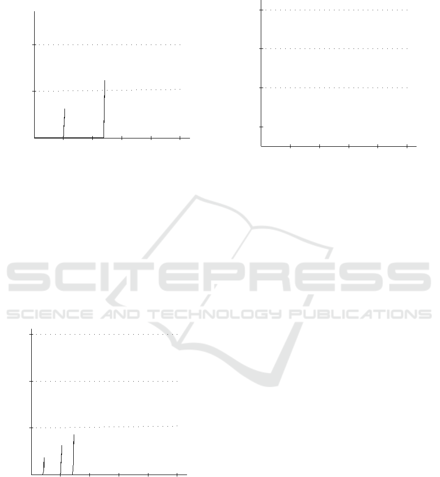
Figure 4 compares the near-optimal allocations

for three different criteria, F2, F10 and F15. When

t = 15, the tangent points are appreciably less than

the baseline case and therefore the 9000 batteries are

enough to supply all the stations with their tangent

points. At this point, all the stations are in their con-

Table 1: The network’s performance for different optimiza-

tion criteria.

Performance Statistic

F2 F5 F10 F15

Criterion

F2 73.5%

1

76.5% 77.5% 77.6%

F5 70.6% 78.6%

2

82.8% 83.2%

F10 49.8% 68.5% 88.5%

3

93.5%

F15 35.0% 54.2% 84.9% 97.9%

4

Notes:

1

Lower bound displayed. The distance between bounds is 0.12%.

2

Lower bound displayed. The distance between bounds is 0.05%.

3

Lower bound displayed. The distance between bounds is 0.02%.

4

Optimal value displayed.

cave region and the residual batteries are distributed

among all the stations. Conversely, when t = 2 the

tangent points are higher than in the baseline case.

Now, the busy stations will demand more batteries to

reach their tangent point and so the budget is depleted

after allocating spares to fewer stations compared to

the baseline case.

6

-

30

60

90

50 100 150 200 250

Number of Batteries

b

l

Station Index

F2

.

......

.

......

.

......

.

......

.

........

.

......

.

......

.

......

.

......

.

......

.

........

.

......

.

......

.

......

.

......

.

........

.

......

.

......

.

......

.

........

.

......

.

......

.

......

.

........

.

......

.

......

.

......

.

........

.

......

.

......

.

......

.

........

.

......

.

......

.

......

.

........

.

......

.

......

.

......

.

........

.

......

.

......

.

F10

.

......

.

........

.

........

.

......

.

........

.

........

.

........

.

......

.

........

.

........

.

........

.

........

.

......

.

........

.

........

.

........

.

........

.

........

.

......

.

........

.

........

.

........

.

........

.

........

.

........

.

........

.

........

.

........

.

........

.

........

.

........

.

........

.

........

.

......

.

........

.

........

.

........

.

........

.

........

.

........

.

........

.

........

.

..........

.

........

.

........

.

........

.

........

.

........

.

........

.

........

.

.....

F15

......

.

........

.

......

.

........

.

......

.

........

.

........

.

........

.

........

.

........

.

......

.

........

.

..........

.

........

.

........

.

........

.

........

.

........

.

........

.

..........

.

........

.

........

.

........

.

..........

.

........

.

........

.

..........

.

........

.

........

.

..........

.

........

.

..........

.

........

.

........

.

..........

.

........

.

..........

.

........

.

..........

.

........

.

..........

.

........

.

..........

.

........

.

..........

.

........

.

..........

.

........

.

..........

.

..........

.

........

.

..........

.

........

.

..........

.

..........

.

........

.

..........

.

..........

.

Figure 4: The spare battery allocation for different opti-

mization criteria.

4.3 The Budget Effect

Figure 5 describes the near-optimal spare allocation

for the baseline case and for spare budgets of 7000

and 11000 batteries. In the baseline scenario, the

number of spare batteries in the network is 9000. If

we increase the budget then the lower-rate stations

will receive batteries one by one according to their

tangent point. Eventually, all the stations will reach

their tangent point. Now, any additional batteries will

be distributed among all the stations instead of given

to only particular stations. In contrast, if the budget

is decreased then some slowest-moving stations will

forfeit all their batteries. The busiest stations, how-

Optimizing Spare Battery Allocation in an Electric Vehicle Battery Swapping System

43

ever, will lose at most the few (if any) batteries they

received beyond their tangent point.

6

-

30

60

50 100 150 200 250

Number of Batteries

b

l

Station Index

B = 7000

F10 = 69.9%

.

........

.

........

.

........

.

........

.

........

.

........

.

......

.

........

.

........

.

........

.

........

.

........

.

........

.

........

.

........

.

........

.

........

.

........

.

........

.

........

.

........

.

........

.

........

.

........

.

........

.

........

.

........

.

........

.

........

.

........

.

..........

.

........

.

B = 9000

F10 = 88.5%

.

......

.

........

.

........

.

......

.

........

.

........

.

........

.

......

.

........

.

........

.

........

.

........

.

......

.

........

.

........

.

........

.

........

.

........

.

......

.

........

.

........

.

........

.

........

.

........

.

........

.

........

.

........

.

........

.

........

.

........

.

........

.

........

.

........

.

......

.

........

.

........

.

........

.

........

.

........

.

........

.

........

.

........

.

..........

.

........

.

........

.

........

.

........

.

........

.

........

.

........

.

.....

B = 11000

F10 = 99.3%

......

.

..

.

......

.

......

.

......

.

......

.

......

.

........

.

......

.

......

.

......

.

......

.

........

.

......

.

......

.

........

.

......

.

........

.

......

.

........

.

......

.

........

.

......

.

........

.

......

.

........

.

......

.

........

.

......

.

........

.

........

.

......

.

........

.

........

.

......

.

........

.

........

.

......

.

........

.

........

.

........

.

......

.

........

.

........

.

........

.

......

.

........

.

........

.

........

.

......

.

........

.

........

.

........

.

........

.

......

.

........

.

........

.

........

.

........

.

........

.

......

.

........

.

........

.

........

.

........

.

........

.

........

.

........

.

......

.

.......

Figure 5: The window ﬁll rate and spare battery allocation

for different values of B.

4.4 The Swapping Time Effect

A corollary of Proposition 1 is that a +∆ change to the

swapping time, t

1

+t

2

is equivalent to a −∆ change to

the tolerable wait, t. Figure 6 shows how the near-

optimal allocation changes with the swapping time.

As the swapping time increases, the tangent points in-

crease too and therefore the busiest stations require

more spares. As a consequence, more and more slow-

moving stations will remain with zero spares.

6

-

30

60

90

50 100 150 200 250

Number of Batteries

b

l

Station Index

t

1

+t

2

=0

F10 = 92.9%

B

t

1

+t

2

=0

........

.

......

.

........

.

........

.

......

.

........

.

........

.

........

.

........

.

........

.

........

.

......

.

........

.

........

.

........

.

........

.

........

.

........

.

........

.

........

.

........

.

........

.

..........

.

........

.

........

.

........

.

........

.

........

.

........

.

........

.

........

.

..........

.

........

.

........

.

........

.

........

.

........

.

..........

.

........

.

........

.

........

.

..........

.

........

.

........

.

........

.

........

.

..........

.

........

.

........

.

..........

.

........

.

........

.

........

.

..........

.

........

.

........

.

t

1

+t

2

=2

F10 = 88.5%



t

1

+t

2

=2

.

......

.

........

.

........

.

......

.

........

.

........

.

........

.

......

.

........

.

........

.

........

.

........

.

......

.

........

.

........

.

........

.

........

.

........

.

......

.

........

.

........

.

........

.

........

.

........

.

........

.

........

.

........

.

........

.

........

.

........

.

........

.

........

.

........

.

......

.

........

.

........

.

........

.

........

.

........

.

........

.

........

.

........

.

..........

.

........

.

........

.

........

.

........

.

........

.

........

.

........

.

.....

t

1

+t

2

=4

F10 = 84.3%

t

1

+t

2

=4

.

......

.

........

.

......

.

........

.

........

.

......

.

........

.

......

.

........

.

........

.

......

.

........

.

........

.

......

.

........

.

........

.

......

.

........

.

........

.

......

.

........

.

........

.

........

.

......

.

........

.

........

.

........

.

......

.

........

.

........

.

........

.

......

.

........

.

........

.

........

.

........

.

......

.

........

.

........

.

........

.

........

.

......

.

........

.

........

.

........

.

........

.

......

.

.....

Figure 6: The spare battery allocation for different battery

swapping times.

Thus far, we assume that the budget of spares is

ﬁxed. Consider, now the dual problem of (6).

min

~

b≥0

L

∑

l=1

b

l

s.t. F(t,

~

b) ≥ α. (8)

where α is the network’s required performance.

6

-

7000

9000

11000

13000

2 4 6 8 10

Spare Battery Budget

B

t

1

+t

2

(minutes)

Swapping Time

F = 90%

slope = 252 batteries/minute

.

F = 95%

slope = 266 batteries/minute

.

F = 99%

slope = 280 batteries/minute

.

Figure 7: The spares budget for different performance target

levels.

We may easily solve (8) using the optimization al-

gorithm. The allocation of spares is done in an identi-

cal manner, but now the stopping condition is that we

have reached the required level of service. Figure 7

displays the budget required to reach a 90%, 95% and

99% window ﬁll rates for different swapping times.

The slope of the graph reveals the savings obtained

by reducing swapping time. For the performance lev-

els of 90%, 95% and 99% the graph is almost linear

and a minute reduction in the swapping time saves

the network approximately 252, 266 and 280 batter-

ies, respectively.

4.5 Optimizing Total Inventory Costs

The problems (6) and (8) assume that either the bud-

get or the service level is predetermined. We now

consider the problem of minimizing the total inven-

tory costs. Let c

B

denote the cost of a battery and let

c

p

denote the penalty cost each time a customer is not

served within the tolerable wait. Since batteries have

a limited lifetime, T , the planning horizon is T and

the total number of customers arriving into the net-

work during the planning horizon is λT where, recall,

λ =

∑

λ

l

. The problem is given by

min

~

b≥0

TC(

~

b) := c

b

L

∑

l=1

b

l

+ c

p

λT



1 − F(t,

~

b)



. (9)

We can easily adjust the optimization algorithm to

ﬁnd the optimal solution to (9). Each time we con-

sider adding a battery we measure its contribution to

the window ﬁll rate, δ. As long as δc

p

λT ≥ c

b

we

increase the number of batteries in the network.

ICORES 2017 - 6th International Conference on Operations Research and Enterprise Systems

44

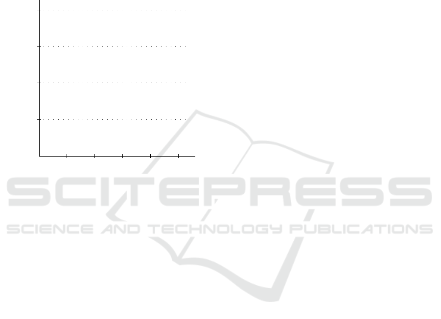
Batteries for family sized electric vehicles range

between 20kWH and 80kWH with current prices

reaching as low as US$200 per-kWh (Sarker et al.,

2015). We therefore examine battery prices of up to

US$25,000. We conservatively estimate battery life

to be four years, and since we assume 12 daily hours

of operation T = 17520 hours (Arcus, 2016). Finally,

the arrival rate to the network is the sum of the arrivals

to all the stations, λ = 14,050 per hour.

6

-

3000

6000

9000

12000

5000 10000 15000 20000 25000

Spare Battery Budget

B

c

b

(US$)

Battery Price

c

p

= $1

.

c

p

= $0.5

.

c

p

= $0.2

.

Figure 8: Spares Budget for different penalty costs and bat-

tery price.

In Figure 8 we depict the near-optimal spares bud-

get depending on battery prices for different penalty

costs. Interestingly, the budget may be very sensi-

tive or very insensitive to battery prices. For exam-

ple, when the penalty is $1, then in the battery price

range of $3261 and $21378 then budget size will only

change between 11000 and 9000 batteries. In stark

contrast, if the price increases from $21378 to only

$25321, then the optimal budget will decrease from

9000 to 0 batteries.

5 CONCLUSIONS

In this paper, we suggest a model to solve the spare

battery allocation problem. Since customers will tol-

erate a certain wait when they enter the station we

claim that to minimize its penalty costs the network

should maximize the fraction of customers who are

served within the tolerable wait, the window ﬁll rate.

We show that the relationship between the win-

dow ﬁll rate when item removal and installment times

are positive to the window ﬁll rate with zero removal

and installment times. Using this relationship, we

build on (Dreyfuss and Giat, 2016) to solve our prob-

lem. To illustrate the application of the model we es-

timate a hypothetical application of a full-scale bat-

tery swapping network in Israel, similar to the net-

work envisioned by the Better Place corporation. Our

numerical analysis of the problem reveals interesting

ﬁndings such as the value of better battery swapping

design, the creation of different classes of stations and

the critical importance of estimating the tolerable wait

correctly.

The model assumes that battery swapping time is

deterministic and that the customer arrival rate is con-

stant over time. While the ﬁrst assumption is reason-

able, the second assumption is clearly unrealistic. We

leave addressing these issues to future research.

REFERENCES

Arcus, C. (2016). Plug-in electric vehicle mar-

ket penetration and incentives: a global re-

view. CleanTechnica. [online] Available at:

https://cleantechnica.com/2016/05/31/battery-

lifetime-long-can-electric-vehicle-batteries-last/

[Accessed 22 Sep. 2016].

Avci, B., Girotra, K., and Netessine, S. (2014). Elec-

tric vehicles with a battery switching station: Adop-

tion and environmental impact. Management Science,

61(4):772–794.

Basten, R. and van Houtum, G. (2014). System-oriented in-

ventory models for spare parts. Surveys in Operations

Research and Management Science, 19(1):34–55.

Berg, M. and Posner, M. (1990). Customer delay in M/G/∞

repair systems with spares. Operations Research,

38(2):344–348.

Bullis, K. (2013). Forget battery swapping: Tesla

aims to charge electric cars in ﬁve minutes.

MIT Technology Review. [online] Available at:

http://www.technologyreview.com/news/516876/forget-

battery-swapping-tesla-aims-to-charge-electric-cars-

in-ﬁve-minutes/ [Accessed 22 Sep. 2016].

Caggiano, K., Jackson, L., Muckstadt, A., and Rappold, A.

(2007). Optimizing service parts inventory in a multi-

echelon, multi-item supply chain with time-based cus-

tomer service-level agreements. Operations Research,

55(2):303–318.

Caggiano, K., Jackson, L., Muckstadt, A., and Rappold,

A. (2009). Efﬁcient computation of time-based cus-

tomer service levels in a multi-item, multi-echelon

supply chain: A practical approach for inventory opti-

mization. European Journal of Operational Research,

199(3):744–749.

Coffman, M., Bernstein, P., and Wee, S. (2016). Electric

vehicles revisited: a review of factors that affect adop-

tion. Transport Review, forthcoming.

Demoulin, N. and Djelassi, S. (2013). Customer responses

to waits for online banking service delivery. Interna-

tional Journal of Retail & Distribution Management,

41(6):442–460.

Optimizing Spare Battery Allocation in an Electric Vehicle Battery Swapping System

45

Dijk, M., Orsato, R., and Kemp, R. (2013). The emer-

gence of an electric mobility trajectory. Energy Policy,

52:135–145.

Dreyfuss, M. and Giat, Y. (2016). Optimal spares allocation

in an exchangeable-item repair system with tolerable

wait. Working Paper, Jerusalem College of Technol-

ogy.

Durrande-Moreau, A. (1999). Waiting for service: ten years

of empirical research. International Journal of Service

Industry Management, 10(2):171–189.

Katz, K., Larson, B., and Larson, R. (1991). Prescriptions

for the waiting in line blues: entertain, enlighten and

engage. Sloan Management Review, (Winter):44–53.

Maister, D. (1985). The psychology of waiting lines. In

Czepiel, J., Solomon, M., and Heath, C. S. D., edi-

tors, The Service Encounter, pages 113–123. Lexing-

ton Books, Lanham, 2nd edition.

Mak, H., Rong, Y., and Shen, Z. (2013). Infrastructure plan-

ning for electric vehicles with battery swapping. Man-

agement Science, 59(7):1557–1575.

Ross, S. (1981). Introduction to probability models. Aca-

demic Press, NY, 2nd edition.

Sarker, M., Hrvoje, P., and Ortega-Vazquez, M. (2015). Op-

timal operation and services scheduling for an electric

vehicle battery swapping station. IEEE Transactions

on Power Systems, 30(2):901–910.

Shtub, A. and Simon, M. (1994). Determination of reorder

points for spare parts in a two-echelon inventory sys-

tem: The case of non-identical maintenance facilities.

European journal of operational research, 73(3):458–

464.

Smidts, A. and Pruyn, A. (1999). How waiting affects cus-

tomer satisfaction with service: the role of subjective

variables. In Proceedings of the 3rd International Re-

search Seminar in Service Management, pages 678–

696. Universite d’Aix-Marseille.

Yang, J. and Sun, H. (2015). Battery swap station location-

routing problem with capacitated electric vehicles.

Computers & Operations Research, 55:217–232.

Zhou, Y., Wang, M., Hao, H., Johnson, L., and Wang, H.

(2015). Plug-in electric vehicle market penetration

and incentives: a global review. Mitigation and Adap-

tation Strategies for Global Change, 20(5):777–795.

ICORES 2017 - 6th International Conference on Operations Research and Enterprise Systems

46