Thrombus Detection in CT Brain Scans using a Convolutional Neural

Network

Aneta Lisowska

1,2

, Erin Beveridge

, Keith Muir

and Ian Poole

Toshiba Medical Visualization Systems Europe Ltd., 2 Anderson Place, Edinburgh, U.K.

School of Engineering and Physical Sciences, Heriot-Watt University, Edinburgh, U.K.

Queen Elizabeth University Hospital, University of Glasgow, Glasgow, U.K.

Keywords:

Convolutional Neural Network, Stroke, Thrombus, Non-contrast Computer Tomography (NCCT).

Abstract:

Automatic detection and measurement of thrombi may expedite clinical workﬂow in the treatment planning

stage. Nevertheless it is a challenging task on non-contrast computed tomography due to the subtlety of

the pathological intensity changes, which are further confounded by the appearance of vascular calciﬁcation

(common in ageing brains). In this paper we propose a 3D Convolutional Neural Network architecture to detect

these subtle signs of stroke. The architecture is designed to exploit contralateral features and anatomical atlas

information. We use 122 CT volumes equally split into training and testing to validate our method, achieving

a ROC AUC of 0.996 and a Precision-Recall AUC of 0.563 in a voxel-level evaluation. The results are not yet

at a level for routine clinical use, but they are encouraging.

1 INTRODUCTION

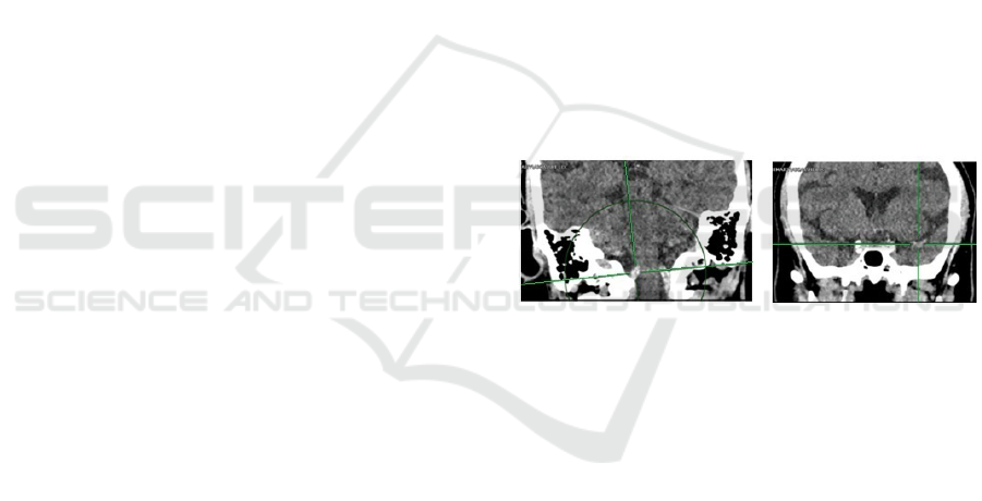
Detection of subtly discriminated regions in volumet-

ric medical imaging is challenging. An example is

the detection of stroke signs in non-contrast computed

tomography (NCCT), where thrombi are one of the

pathologies of interest. Thrombi manifest as subtle

vascular intensity and texture changes which are chal-

lenging to identify due to the proximity of bone, and

the similarity to normal age related vascular calciﬁca-

tion (see Figure 1).

Automatic detection of thrombi and their subse-

quent measurements may provide information which

is important for treatment planning. For example, the

length of the thrombus observed in thin slice NCCT is

related to the success rate of thrombolysis, a treatment

aimed to recanalise occluded arteries (Riedel et al.,

2011). Nevertheless, to our knowledge, the problem

of automatic thrombus detection has not been directly

addressed.

Detection of stroke signs in CT scans has previ-

ously been demonstrated at the brain level. Chawla

et al. proposed a general system for classiﬁcation

of ischaemic and haemorrhagic stroke signs (Chawla

et al., 2009). Their system computes a separate his-

togram of intensity values for each hemisphere, and

the classiﬁcation of the image slice is based on the

comparison between the left and right histograms.

The authors report good performance in determining

the type of stroke, but the system is not designed to

Figure 1: Left: Normal calciﬁcation of arteries, which could

be confused with abnormal dense vessel signs. Right: Ex-

ample of a CT brain scan with a clearly visible dense vessel.

give a precise location of the stoke sign. Furthermore

the haemorrhage is easily detectable on CT compared

to ischaemia or thrombus.

Precise location of stroke signs requires a more lo-

calised model. One approach is to compare the patient

image with a normative atlas created from healthy ex-

amples of anatomy; the patient image is registered to

the normative atlas and the pathology is identiﬁed by

the differences between the reference atlas and the ex-

amined image (Doyle et al., 2013). This approach re-

quires accurate non-rigid registration, which may not

always be possible due to anatomical variability. Ma-

chine learning algorithms are one method of learning

diverse non-parametric appearance models. For in-

stance, random forest classiﬁers have been success-

fully applied to various medical imaging segmenta-

tion tasks (Geremia et al., 2011; Zikic et al., 2012).

However, in recent years CNN-based solutions have

dominated brain image analysis applications, result-

ing in the best performance in the Ischemic Stroke Le-

Lisowska A., Beveridge E., Muir K. and Poole I.

Thrombus Detection in CT Brain Scans using a Convolutional Neural Network.

DOI: 10.5220/0006114600240033

In Proceedings of the 10th International Joint Conference on Biomedical Engineering Systems and Technologies (BIOSTEC 2017), pages 24-33

ISBN: 978-989-758-215-8

sion Segmentation (ISLES) (winning solution in 2015

(Kamnitsas et al., 2016)) and Brain Tumor Segmenta-

tion (BRATS) challenges (see CNN based application

(Havaei et al., 2016) (Pereira et al., 2015)). These

CNN solutions are trained on brain MRI data, how-

ever CNNs have also been applied to CT images of the

knee (Prasoon et al., 2013) and lungs (Anthimopoulos

et al., 2016). The CNN architecture design may differ

between the imaging modalities and between various

anatomies of interest. (Li et al., 2014) observe that CT

images lack structural detail in regions of soft tissue,

taking on a textured appearance, therefore there are

few higher-level concepts for a deep network to learn.

Prasoon et al. also avoided use of deep architecture

in CT and pointed out that thin structure of cartilage

can be lost if too many mean-pooling layers are ap-

plied (Prasoon et al., 2013). In this paper we employ

a fully convolutional architecture, which is only 7 lay-

ers deep as described in Section 2.

CT scans are three-dimensional (3D), and there-

fore architectures designed for images cannot be di-

rectly applied. When moving to 3D data, three strate-

gies are common. Firstly, the volume may be treated

as a stack of 2D slices on which a 2D architecture

is directly applied. Volumes are often acquired in

a slice-wise manner, and where the slice spacing is

large, this may be a natural approach. The second

strategy is a triplanar CNN (Prasoon et al., 2013;

Yang et al., 2015) in which axial, sagittal and coro-

nal slices centred at the voxel of interest are consid-

ered separately and fed to three 2D CNNs (or three

channels of a 2D CNN (Roth et al., 2014; Wolterink

et al., 2015)). Their outputs are combined in the pre-

classiﬁcation stage. Finally, 3D convolution (Urban

et al., 2014; Kamnitsas et al., 2015; Payan and Mon-

tana, 2015) may be used in place of 2D convolution.

This last strategy is computationally expensive, thus

training and optimisation of a network can be ardu-

ous. Payan and Montana compared a 2D CNN with

a 3D CNN on brain MRI data and found that the 3D

CNN obtained marginally better Alzheimer classiﬁca-

tion accuracy (Payan and Montana, 2015). In this pa-

per we adopt a 3D CNN, but we apply spatial decom-

position of the kernels to address the computational

complexity issue such that convolutions are applied

one dimension at the time.

A key element of our architecture is bilateral fea-

ture comparison. The idea of bilateral feature compar-

ison is strongly linked with exploitation of anatom-

ical symmetry, which has been also incorporated in

unsupervised approaches of pathology detection. Re-

searchers utilised in-organ symmetry for detection of

tumours in the brain (Hasan et al., 2016; Zhao et al.,

2013) and prostate (Qiu et al., 2013). There have also

been attempts to examine symmetry between a pair of

organs in breast tumour detection (Erihov et al., 2015;

Bandyopadhyay, 2010). In these approaches, the

pathology is found by searching for the most dissimi-

lar regions between the left and right side of the organ

(Hasan et al., 2016), or by identiﬁcation of asymmetry

between paired organs (Erihov et al., 2015). It is rare

that a stroke will occur in both sides of the brain in

a given episode, therefore comparison between hemi-

spheres helps to discriminate between subtle changes

in the affected side and the normal brain tissue. We

hypothesise that exploiting contralateral features will

therefore be useful when detecting thrombi.

The second key element of our architecture is the

explicit incorporation of spatial anatomical context by

provision of the coordinates in a (rigidly-registered)

reference dataset “atlas” by adding three channels

encoding x, y, z atlas locations. In this, we fol-

low the lead of authors such as (O’Neil et al., 2015)

who used atlas coordinates as a feature provided to

a random forest when learning to detect anatomi-

cal landmarks. The injection of contextual informa-

tion into a machine learning algorithm was demon-

strated in a traumatic brain injury application by (Rao

et al., 2014) who used multi-atlas propagation and

EM (MALPEM) (Ledig et al., 2012) to obtain tissue

classes priors which were later exploited in a random

forest. Since the thrombi may be subtle, the addition

of anatomical context might provide a helpful insight.

One of the challenges in training a CNN to de-

tect thrombus is the signiﬁcantly limited set of sam-

ples containing pathology compared to healthy tis-

sue. As a result, the CNN may take little account of

the underrepresented class during training. One solu-

tion to address this problem is to alter the loss func-

tion. For neutrophil detection, (Wang et al., 2015)

penalised more heavily the misclassiﬁcation of non-

neutrophils than that of neutrophils, by doubling the

computed softmax loss. (Brosch et al., 2015) de-

signed a specialised CNN objective function which

relies on a weighted combination of sensitivity and

speciﬁcity. A more mechanical approach is to take

all samples from the underrepresented category and a

random subset of the examples from the other cate-

gory (Ciresan et al., 2012; Roth et al., 2014; Li et al.,

2015; Rao et al., 2015). However, random sampling

of classes may not always give the most useful train-

ing distribution. A number of papers deliberately bi-

ased the training distribution towards examples which

were more difﬁcult to classify due to visual proxim-

ity between classes. Researchers commonly sampled

background more densely close to the region of in-

terest compared to other areas (Ciresan et al., 2013;

Prasoon et al., 2013; Dvorak and Menze, 2015). Re-

Thrombus Detection in CT Brain Scans using a Convolutional Neural Network

cently, (Kamnitsas et al., 2016) suggested that train-

ing on large image segments allows for automatic ad-

justment to this problem. In this paper we choose to

use a weighting function to compensate for the unbal-

anced sample distribution such that normal and abnor-

mal samples count equally in the loss function.

In summary, this paper makes three contributions:

• We propose a 3D CNN architecture incorporating

brain symmetry exploitation and atlas information

( Section 2). We present qualitative and quanti-

tative results obtained by applying the proposed

CNN to the thrombus detection problem ( Section

4.2).

• As far as we are aware, this is the ﬁrst CNN-based

solution applied to brain NCCT and the ﬁrst solu-

tion for automatic thrombus detection.

• We study the effect of the training procedure on

efﬁciency. We compare patch and segment based

training to full block training with and without

weighting of the loss function in order to identify

the most effective training strategy in an unbal-

anced sample setting ( Section 4.1).

2 METHODS

We propose a convolutional neural network (CNN)

which leverages left and right hemisphere compari-

son (See Figure 3). The ﬁrst steps consist of isotropic

resampling to 1mm voxels and alignment of the CT

volumes to a reference dataset designated as an atlas.

The transformation between a given dataset and a ref-

erence atlas is discovered via landmarks, which are

detected in the novel volume by random forest as pro-

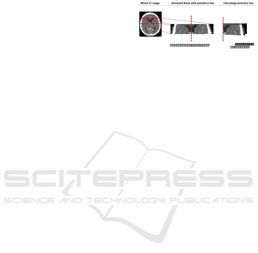
posed in (Dabbah et al., 2014). A block of interest

extending into the sagittal plane is then extracted and

folded along the brain midline, similarly to the fold-

ing of a butterﬂy’s wings (see Figure 2). This folding

results in two 3D CNN intensity channels relating to

the target and contralateral sides of the brain, enabling

bilateral comparison. We call this architecture a But-

terﬂy CNN. Since the architecture works in the folded

space, it is left-right agnostic with respect to the tar-

get laterality. The target and contralateral channels

may thus correspond to either left and right, or right

and left, respectively. Consequently there is sharing

of training data between left and right hemispheres.

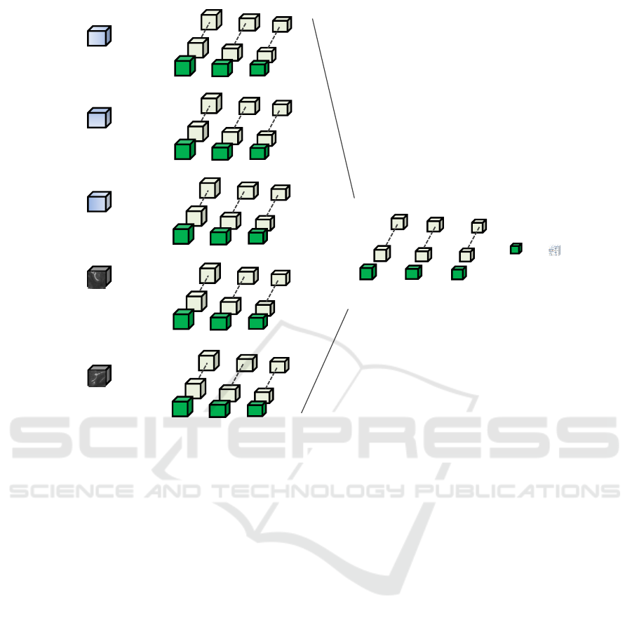
Alongside the two data input channels, we insert

three channels encoding the x, y and z atlas coordi-

nates to the architecture. For the convolution opera-

tions, we use a spatial decomposition of a 5x5x5 ﬁl-

ter e.g. three layers of orthogonal one-dimensional

convolutions: 5x1x1, 1x5x1, 1x1x5. N

= 32 ker-

Figure 2: Block extraction.

nels are used for the data channels and N

= 4 ker-

nels are used for the atlas channels. Channels are then

merged and another convolution operation is applied,

with N

= 32 kernels. See Figure 3 for a diagram of

the architecture. ReLU activation functions are used.

The output is fully convolutional allowing for the efﬁ-

cient prediction of all voxels of the dataset in a single

pass.

The model was implemented in Python using the

Keras library built on top of Theano. Training was

performed using stochastic gradient descent on nor-

malised data samples, with learning rate 0.001, op-

timising the squared hinge loss function, momentum

0.9 and L2 regularisation 0.002.

3 MATERIALS

We use data from the South Glasgow Stroke Imag-

ing Database, which includes the following studies:

ATTEST (Huang et al., 2015), POSH and WYETH

(Wardlaw et al., 2013) provided by the Institute of

Neuroscience and Psychology, University of Glas-

gow, Southern General Hospital. Ground truth was

collected on the acute non-contrast CT (NCCT) scan

for 122 patients with suspected acute ischaemic stroke

within 6 hours of onset. Manual segmentations of

thrombi were generated in 3D Slicer 4.5.0 by a clin-

ical researcher under the supervision of an experi-

enced neuroradiologist. Annotations were blind to

additional scans (e.g. CT angiography, CT perfusion,

follow-up scans) and clinical information with the ex-

ception of the laterality of the symptoms. Current

methods are applied only to the anterior circulation

but consider both proximal occlusions and more dis-

tal dot signs.

There might be some uncertainty around precise

segmentation of the thrombi. Since we are interested

only in detection, it is undesirable for the network to

waste learning capacity trying to reﬁne the boundary.

We consider a border, 2mm in width around each ab-

normality, as a “do not care” zone. Such voxels do not

inﬂuence the loss function which drives the stochastic

gradient descent, nor are they included in the results.

BIOIMAGING 2017 - 4th International Conference on Bioimaging

abs(x)

CNN Input

1 @ 1 x 1 x 1

CNN Output

𝑁

𝑀

@ 5 x 1 x 1

𝑁

𝑀

@ 1 x 5 x 1 𝑁

𝑀

@ 1 x 1 x 5

Target

laterality

Comparative

laterality

Prediction

for target

laterality

𝑁

𝐼

@ 5 x 1 x 1

𝑁

𝐼

@ 1 x 5 x 1 𝑁

𝐼

@ 1 x 1 x 5

𝑁

𝐴

@ 5 x 1 x 1 𝑁

𝐴

@ 1 x 5x 1 𝑁

𝐴

@ 1 x 1 x 5

𝑁

𝐴

@ 5 x 1 x 1

𝑁

𝐴

@ 1 x 5x 1

𝑁

𝐴

@ 1 x 1 x 5

𝑁

𝐴

@ 5 x 1 x 1 𝑁

𝐴

@ 1 x 5x 1

𝑁

𝐴

@ 1 x 1 x 5

𝑁

𝐼

@ 5 x 1 x 1

𝑁

𝐼

@ 1 x 5 x 1 𝑁

𝐼

@ 1 x 1 x 5

Figure 3: Schematic of the CNN architecture.

For implementation, we use -1 and +1 to represent

normal and thrombi voxels respectively, and use the

value 0 to represent the ”do not care” voxels. The

border zone is constructed using morphological dila-

tion.

For training and testing of the CNN classiﬁer we

used a Titan X GPU.

4 EXPERIMENTS

The data was split equally (and randomly) into 61

training datasets and 61 testing datasets.

We evaluated the performance of the CNN in Sec-

tion 4.2 in terms of the area under the curve (AUC)

for the Receiver Operating Curve (ROC AUC) and

the precision-recall (PR AUC) curve. The ROC curve

represents the relationship between sensitivity (i.e. re-

call) and speciﬁcity, while the PR curve represents the

relationship between precision and recall. Sensitiv-

ity (recall) is a measure of how many of the positive

samples have been correctly identiﬁed as being pos-

itive. Speciﬁcity is a measure of how many of the

negative samples have been correctly identiﬁed as be-

ing negative. Precision is a measure of how many of

the samples predicted by the classiﬁer as positive are

indeed positive. It is suggested that PR curves should

be used when the positive class samples are rare com-

pared to the negative class samples (Davis and Goad-

rich, 2006), because precision is more sensitive to any

change in the number of false positives, while speci-

ﬁcity is not due to the large number of negative sam-

ples. As an example, if the ratio of normal to abnor-

mal is 10, 000 : 1 then even a false positive rate of

0.01 results in 100 false detections.

4.1 Patch vs. Full Block Training

In our efforts to establish the most efﬁcient train-

ing procedure, we compare training of the CNN with

whole blocks as input versus training with small

patches as input. We introduce a weighting factor w to

allow for the correction of the imbalance between nor-

mal and abnormal samples. We deﬁne w as the ratio

of normal to abnormal voxels in the training set. The

CNN architecture as presented in Figure 3 is used, but

with smaller ﬁlter size 3x3x3 and trained only for 250

epochs. We are primarily interested in the training

time of the network, but we also report PR AUC to

ensure the learning took place.

Thrombus Detection in CT Brain Scans using a Convolutional Neural Network

Figure 4: 2D representation of biased patch selection pro-

cess. More patches of abnormality than normality are se-

lected, in order to compensate for the presence of normal

voxels within the abnormal patches, to achieve a balanced

training set. The green box represents the ﬁeld of view (a

margin) and the blue box is the core patch size, for which

predictions are being output during training.

For the patch training, we sample equal numbers

of normal and abnormal locations, but we vary the

size of the core patch that we extract at each location.

The core size corresponds to the voxels for which the

response is computed. In practice, we require a larger

input patch to the network, in order to include a mar-

gin of voxels for which the ﬁlter response is not com-

puted, as we employ valid-mode convolutional oper-

ations. In one dimension and input patch size P, con-

volving with ﬁlter F will produce a feature map M of

size P − F + 1. Therefore, to produce an output of

1 voxel after 2 convolutions with ﬁlter size 3 in each

dimension, the input patch size is 5

. The core patch

size of 1 will have samples only from one class, never-

theless inputs with a larger core patch size are likely

to have voxels from both classes when an abnormal

patch is extracted (See Figure 4. This case resembles

the image segment training procedure of (Kamnitsas

et al., 2016). The results obtained for 3 different in-

put patch sizes and full folded block training are pre-

sented in Table 1.

We found that full block training took signiﬁcantly

longer than patch-based training. It is evident that

weighting of the loss function is necessary to compen-

sate any severe imbalance of training data samples, as

is the case when the CNN is trained on the full block

or large patches. For the core patch size 1

, no learn-

ing occurred when using either a weighted or an un-

weighted loss function. It might be due to exposure

of the network to insufﬁcient number of training vox-

els, which is not a problem when trained on the larger

patches. The network trained on core patch size 1

might not have seen the difﬁcult examples which are

close to the lesion borders, which would always be

included when training on the larger patches.

In a further experiment we train the CNN on large

patches with a weighted loss function. This allows for

efﬁcient training without the need for extensive ex-

perimentation to select an appropriate patch size, for

which weighting of the loss function is not required.

Table 1: The table shows the precision-recall AUC achieved

on a test dataset after just 250 epochs of training and cor-

responding training time. PBT (Patch based training), FBT

(Full Block Training), PBTw (Patch based training with loss

function weighting), FBTw (Full Block Training with loss

function weighting).

Method Precision-

Recall AUC

Training

time

PBT (core patch 1) 0.015 1.50 h

PBTw (core patch 1) 0.023 1.52 h

PBT (core patch 5) 0.341 29.3 min

PBTw(core patch 5) 0.320 29.4 min

PBT (core patch 10) 0.006 36.4 min

PBTw (core patch 10) 0.347 36.2 min

FBT 0.002 16.7 h

FBTw 0.397 16.6 h

4.2 Thrombus Detection Results

The CNN detector (as presented in Figure 3) was

trained for 800 epochs on input patches of size 24

(core patch 16

) extracted from 61 training datasets.

The detector was evaluated on 61 testing datasets

and the quantitative results are presented in Table 2.

Training took 2.15h and detection time/ per block is

4s.

For comparison we trained also a simple CNN net-

work which is composed from 7 layers and the num-

ber of kernels and ﬁlter sizes are the same as in the

Figure 3 the difference is that it has only one input

channel. The bilateral comparison and atlas informa-

tion is not incorporated in the simple CNN.

The precision-recall curves for both the simple

and the Butterﬂy CNNs are shown in Figure 5 and

the ROC for the Butterﬂy CNN is shown in Figure

6. Some example detection results are presented in

Figure 7 and Figure 8. The former show a case of

very subtle thrombus where we fail to detect it at the

sagittal slice of the abnormality and quite a few false

positives are visible in the maximum intensity pro-

jection (MIP) view. The latter is more clearly visible

thrombus and the detections are almost perfect.

Table 2: Thrombus detection evaluation.

Model ROC AUC Precision-

Recall AUC

Butterﬂy

CNN

0.997 0.562

Simple CNN 0.996 0.178

BIOIMAGING 2017 - 4th International Conference on Bioimaging

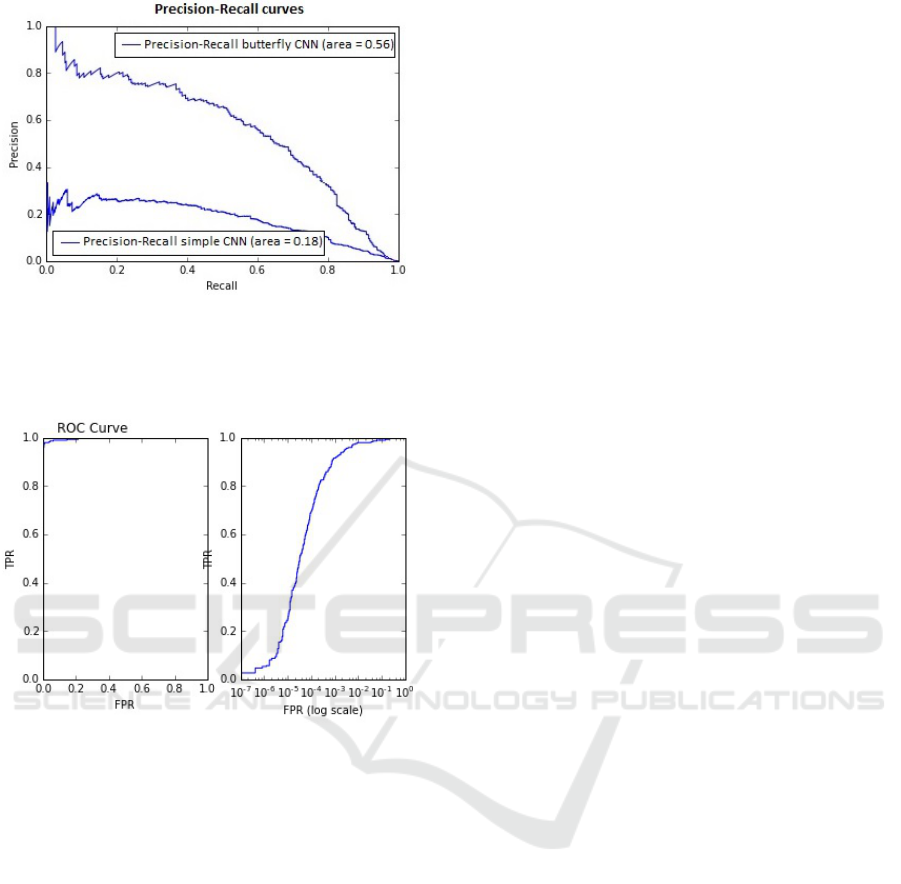
Figure 5: Precision-Recall curves for Simple CNN and But-

terﬂy CNN. At the point that around 70% of thrombi are

detected the simple CNN would give around 20% true de-

tection results whereas the Butterﬂy CNN would produce

just above 50% of true detection results.

Figure 6: Left: ROC curve in full. Right: ROC curve shown

with a log scale on the speciﬁcity axis, to focus on the range

of interest. For the thrombus detector to be clinically useful

the false positive rate at the voxel level needs to be very low,

of order 10

−4

or better, otherwise false positive detections

will overwhelm true positives.

5 DISCUSSION

We have found that weighting of the loss function to

compensate for unbalanced training data is effective,

even essential, when training either on the full block

or using a large image patches. Patch-based training

is signiﬁcantly faster than full block training. The

downside of this approach is that it requires careful

selection of the size of the patches when the weighting

of the loss function is not applied. To overcome this

difﬁculty we have adapted the combination of larger

path and weighting of the loss function for training of

the thrombus detector.

The quantitative and visual results obtained us-

ing presented solution are encouraging. However, to

reach detection performance level at which the detec-

tor could be applied clinically the number of the false

positive detections needs to be further reduced. To

achieve this we will consider adapting a cascade ap-

proach similar to boosting, so that a second classiﬁer

is trained only on on normal examples which were

misclassiﬁed at the ﬁrst detection stage, this might

help to eliminate false positive detections (Liswoska

et al., 2016).

The proposed architecture for thrombus detection

performs better than a single channel CNN. This sup-

ports our hypothesis that incorporation of atlas in-

formation and bilateral features within the CNN ar-

chitecture is helpful when identifying subtle stroke

signs. In future experiments it would be interesting to

evaluate the extent to which each of the architectural

choices contribute to the thrombus detection perfor-

mance and whether the level at which they are in-

serted to the CNN architecture affects their useful-

ness.

Large amount of medical imaging data is difﬁ-

cult to obtain, especially given the requirement for

ground truth labels provided by expert clinicians. Re-

searchers have tried to address this problem by us-

ing transfer learning. In this scheme a network ﬁrst

trained on large annotated natural image datasets like

ImageNet, followed by ﬁne-tuning on the smaller

medical imaging dataset. (Shin et al., 2016) found this

approach to be beneﬁcial when applied to both tho-

racoabdominal lymph node detection and interstitial

lung disease classiﬁcation in CT scans. On the other

hand (Arevalo et al., 2015) and (Gao et al., 2016)

found that CNN models trained fully with the domain

images performed better than models pretrained on

the ImageNet dataset when applied to the problems

of mammography mass lesion classiﬁcation and Inter-

stitial Lung Disease Pattern Detection in CT respec-

tively. It is unclear if this training approach would be

helpful for thrombus detection; further investigation

is required. An interesting avenue to explore might

be knowledge transfer between two medical image

datasets or alternatively between two different tasks.

We hypothesise that the proposed CNN architec-

ture would also be well suited to the detection of other

stoke signs and we plan to train it on ischaemic re-

gions in future study. This will provide an opportu-

nity to evaluate beneﬁts coming from within-domain

transfer learning. The model trained purely on is-

chaemic data can be compared to the thrombus detec-

tion model ﬁne-tuned for ischaemia detection prob-

lems.

Future assessment of the detector performance

will also include patient level evaluation and testing

on more brain CT datasets from different institutions.

Thrombus Detection in CT Brain Scans using a Convolutional Neural Network

Figure 7: Top to bottom: CT image at the abnormal slice, ground truth segmentations at the abnormal slice (here: gray region

is a ”do not care” zone), detection at the abnormal slice (note misdetection in a sagittal slice), ground truth in a projection

view through the whole volume, detection in a projection through the volume (a few false positive detections are present).

BIOIMAGING 2017 - 4th International Conference on Bioimaging

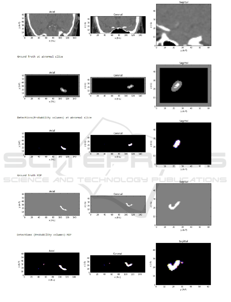
Figure 8: Top to bottom: CT image at the abnormal slice (** note posterior top, anterior bottom of the CT image) with

thrombus clearly visible, ground truth segmentations at the abnormal slice (here:gray region is a ”do not care” zone), detection

at the abnormal slice (clear detection), ground truth in a projection view through the whole volume, detection in a projection

through the volume (a few false positive detections are present, but with lower certainty (dark blue and yellow colors as

opposed to bright white true positive detections).

Thrombus Detection in CT Brain Scans using a Convolutional Neural Network

6 CONCLUSION

We have proposed a CNN for thrombus detection

in brain CT. The suggested architecture utilises con-

tralateral features and atlas information. The method

is evaluated at the voxel level on 61 NCCT datasets

and some example detection results are presented.

Both quantitative and visual results are encouraging.

Further investigation, as mentioned in the discussion,

may lead to improvement of the detector to a level at

which it could be applied in the clinical setting.

ACKNOWLEDGEMENTS

We wish to thank Alison O’Neil for her helpful com-

ments on the manuscript draft.

REFERENCES

Anthimopoulos, M., Christodoulidis, S., Ebner, L., Christe,

A., and Mougiakakou, S. (2016). Lung pattern classi-

ﬁcation for interstitial lung diseases using a deep con-

volutional neural network. IEEE transactions on med-

ical imaging, 35(5):1207–1216.

Arevalo, J., Gonzalez, F. A., Ramos-Pollan, R., Oliveira,

J. L., and Guevara Lopez, M. A. (2015). Convolu-

tional neural networks for mammography mass lesion

classiﬁcation. In Engineering in Medicine and Biol-

ogy Society (EMBC), 2015 37th Annual International

Conference of the IEEE, pages 797–800. IEEE.

Bandyopadhyay, S. K. (2010). Breast asymmetry-tutorial

review. Breast, 9(8).

Brosch, T., Yoo, Y., Tang, L. Y., Li, D. K., Traboulsee,

A., and Tam, R. (2015). Deep convolutional encoder

networks for multiple sclerosis lesion segmentation.

In Medical Image Computing and Computer-Assisted

Intervention–MICCAI 2015, pages 3–11. Springer.

Chawla, M., Sharma, S., Sivaswamy, J., and Kishore, L.

(2009). A method for automatic detection and classi-

ﬁcation of stroke from brain ct images. In Engineering

in Medicine and Biology Society, volume 2009, pages

3581–3584.

Ciresan, D., Giusti, A., Gambardella, L. M., and Schmid-

huber, J. (2012). Deep neural networks segment neu-

ronal membranes in electron microscopy images. In

Advances in neural information processing systems,

pages 2843–2851.

Ciresan, D. C., Giusti, A., Gambardella, L. M., and Schmid-

huber, J. (2013). Mitosis detection in breast cancer

histology images with deep neural networks. Lecture

Notes in Computer Science (including subseries Lec-

ture Notes in Artiﬁcial Intelligence and Lecture Notes

in Bioinformatics), 8150 LNCS(PART 2):411–418.

Dabbah, M. A., Murphy, S., Pello, H., Courbon, R., Bev-

eridge, E., Wiseman, S., Wyeth, D., and Poole, I.

(2014). Detection and location of 127 anatomical

landmarks in diverse ct datasets. In SPIE Medical

Imaging, pages 903415–903415. International Society

for Optics and Photonics.

Davis, J. and Goadrich, M. (2006). The relationship be-

tween precision-recall and roc curves. In Proceed-

ings of the 23rd International Conference on Machine

Learning, ICML’06, pages 233–240.

Doyle, S., Vasseur, F., Dojat, M., and Forbes, F. (2013).

Fully automatic brain tumor segmentation from multi-

ple mr sequences using hidden markov ﬁelds and vari-

ational em. Procs. NCI-MICCAI BraTS, pages 18–22.

Dvorak, P. and Menze, B. (2015). Structured prediction

with convolutional neural networks for multimodal

brain tumor segmentation. Proceedings of BRATS-

MICCAI.

Erihov, M., Alpert, S., Kisilev, P., and Hashoul, S. (2015).

A cross saliency approach to asymmetry-based tumor

detection. In International Conference on Medical Im-

age Computing and Computer-Assisted Intervention,

pages 636–643. Springer.

Gao, M., Xu, Z., Lu, L., Harrison, A. P., Summers, R. M.,

and Mollura, D. J. (2016). Multi-label deep regression

and unordered pooling for holistic interstitial lung dis-

ease pattern detection. In International Workshop on

Machine Learning in Medical Imaging, pages 147–

155. Springer.

Geremia, E., Clatz, O., Menze, B. H., Konukoglu, E., Cri-

minisi, A., and Ayache, N. (2011). Spatial decision

forests for ms lesion segmentation in multi-channel

magnetic resonance images. NeuroImage, 57(2):378–

390.

Hasan, A., Meziane, F., and Khadim, M. (2016). Auto-

mated segmentation of tumours in mri brain scans. In

Proceedings of the 9th International Joint Conference

on Biomedical Engineering Systems and Technologies

(BIOSTEC 2016), pages 55–62. SCITEPRESS.

Havaei, M., Davy, A., Warde-Farley, D., Biard, A.,

Courville, A., Bengio, Y., Pal, C., Jodoin, P.-M., and

Larochelle, H. (2016). Brain tumor segmentation with

deep neural networks. Medical Image Analysis.

Huang, X., Cheripelli, B. K., Lloyd, S. M., Kalladka, D.,

Moreton, F. C., Siddiqui, A., Ford, I., and Muir, K. W.

(2015). Alteplase versus tenecteplase for thrombol-

ysis after ischaemic stroke (attest): a phase 2, ran-

domised, open-label, blinded endpoint study. The

Lancet Neurology, 14(4):368–376.

Kamnitsas, K., Chen, L., Ledig, C., Rueckert, D., and

Glocker, B. (2015). Multi-scale 3D convolutional neu-

ral networks for lesion segmentation in brain MRI. Is-

chemic Stroke Lesion Segmentation, page 13.

Kamnitsas, K., Ledig, C., Newcombe, V. F., Simpson,

J. P., Kane, A. D., Menon, D. K., Rueckert, D., and

Glocker, B. (2016). Efﬁcient multi-scale 3d cnn with

fully connected crf for accurate brain lesion segmen-

tation. arXiv preprint arXiv:1603.05959.

Ledig, C., Wolz, R., Aljabar, P., L

otj

onen, J., Hecke-

mann, R. A., Hammers, A., and Rueckert, D. (2012).

Multi-class brain segmentation using atlas propaga-

tion and em-based reﬁnement. In 2012 9th IEEE Inter-

BIOIMAGING 2017 - 4th International Conference on Bioimaging

national Symposium on Biomedical Imaging (ISBI),

pages 896–899. IEEE.

Li, Q., Cai, W., Wang, X., Zhou, Y., Feng, D. D., and

Chen, M. (2014). Medical image classiﬁcation with

convolutional neural network. In Control Automation

Robotics & Vision (ICARCV), 2014 13th International

Conference on, pages 844–848. IEEE.

Li, W., Jia, F., and Hu, Q. (2015). Automatic segmentation

of liver tumor in CT images with deep convolutional

neural networks. Journal of Computer and Communi-

cations, 3(11):146.

Liswoska, A., Beveridge, E., and Poole, I. (2016). False

positive reduction methods applied to dense vessel de-

tection in brain ct images. Poster presented at Medical

Imaging Summer School, Favigana, Italy.

O’Neil, A., Murphy, S., and Poole, I. (2015). Anatomical

landmark detection in ct data by learned atlas location

autocontext. In MIUA, pages 189–194.

Payan, A. and Montana, G. (2015). Predicting alzheimer’s

disease: a neuroimaging study with 3d convolutional

neural networks. arXiv preprint arXiv:1502.02506.

Pereira, S., Pinto, A., Alves, V., and Silva, C. A. (2015).

Deep convolutional neural networks for the segmen-

tation of gliomas in multi-sequence mri. In Inter-

national Workshop on Brainlesion: Glioma, Multiple

Sclerosis, Stroke and Traumatic Brain Injuries, pages

131–143. Springer.

Prasoon, A., Petersen, K., Igel, C., Lauze, F., Dam, E.,

and Nielsen, M. (2013). Deep feature learning for

knee cartilage segmentation using a triplanar convolu-

tional neural network. In Medical Image Computing

and Computer-Assisted Intervention–MICCAI 2013,

pages 246–253. Springer.

Qiu, W., Yuan, J., Ukwatta, E., Sun, Y., Rajchl, M., and Fen-

ster, A. (2013). Fast globally optimal segmentation

of 3d prostate mri with axial symmetry prior. In In-

ternational Conference on Medical Image Computing

and Computer-Assisted Intervention, pages 198–205.

Springer.

Rao, A., Ledig, C., Newcombe, V., Menon, D., and Rueck-

ert, D. (2014). Contusion segmentation from subjects

with traumatic brain injury: a random forest frame-

work. In 2014 IEEE 11th International Symposium

on Biomedical Imaging (ISBI), pages 333–336. IEEE.

Rao, V., Sarabi, M. S., and Jaiswal, A. (2015). Brain tu-

mor segmentation with deep learning. Proceedings of

BRATS-MICCAI.

Riedel, C. H., Zimmermann, P., Jensen-Kondering, U., Stin-

gele, R., Deuschl, G., and Jansen, O. (2011). The

importance of size successful recanalization by intra-

venous thrombolysis in acute anterior stroke depends

on thrombus length. Stroke, 42(6):1775–1777.

Roth, H. R., Lu, L., Seff, A., Cherry, K. M., Hoffman, J.,

Wang, S., Liu, J., Turkbey, E., and Summers, R. M.

(2014). A new 2.5 D representation for lymph node

detection using random sets of deep convolutional

neural network observations. In Medical Image Com-

puting and Computer-Assisted Intervention–MICCAI

2014, pages 520–527. Springer.

Shin, H.-C., Roth, H. R., Gao, M., Lu, L., Xu, Z., Nogues,

I., Yao, J., Mollura, D., and Summers, R. M. (2016).

Deep convolutional neural networks for computer-

aided detection: Cnn architectures, dataset charac-

teristics and transfer learning. IEEE transactions on

medical imaging, 35(5):1285–1298.

Urban, G., Bendszus, M., Hamprecht, F., and Kleesiek, J.

(2014). Multi-modal brain tumor segmentation using

deep convolutional neural networks. Proceedings of

BRATS-MICCAI.

Wang, J., MacKenzie, J. D., Ramachandran, R., and Chen,

D. Z. (2015). Neutrophils identiﬁcation by deep learn-

ing and voronoi diagram of clusters. In Medical Im-

age Computing and Computer-Assisted Intervention–

MICCAI 2015, pages 226–233. Springer.

Wardlaw, J. M., Muir, K. W., Macleod, M.-J., Weir, C.,

McVerry, F., Carpenter, T., Shuler, K., Thomas, R.,

Acheampong, P., Dani, K., et al. (2013). Clinical rele-

vance and practical implications of trials of perfusion

and angiographic imaging in patients with acute is-

chaemic stroke: a multicentre cohort imaging study.

Journal of Neurology, Neurosurgery & Psychiatry,

pages jnnp–2012.

Wolterink, J. M., Leiner, T., Viergever, M. A., and I

sgum,

I. (2015). Automatic coronary calcium scoring in car-

diac CT angiography using convolutional neural net-

works. In Medical Image Computing and Computer-

Assisted Intervention–MICCAI 2015, pages 589–596.

Springer.

Yang, D., Zhang, S., Yan, Z., Tan, C., Li, K., and Metaxas,

D. (2015). Automated anatomical landmark detection

on distal femur surface using convolutional neural net-

work. In Biomedical Imaging (ISBI), 2015 IEEE 12th

International Symposium on, pages 17–21. IEEE.

Zhao, L., Wu, W., and Corso, J. J. (2013). Semi-automatic

brain tumor segmentation by constrained mrfs using

structural trajectories. In International Conference on

Medical Image Computing and Computer-Assisted In-

tervention, pages 567–575. Springer.

Zikic, D., Glocker, B., Konukoglu, E., Criminisi, A., Demi-

ralp, C., Shotton, J., Thomas, O., Das, T., Jena, R.,

and Price, S. (2012). Decision forests for tissue-

speciﬁc segmentation of high-grade gliomas in multi-

channel mr. In International Conference on Medi-

cal Image Computing and Computer-Assisted Inter-

vention, pages 369–376. Springer.

Thrombus Detection in CT Brain Scans using a Convolutional Neural Network