Variable Neighbourhood Search Solving Sub-problems of a Lagrangian

Flexible Scheduling Problem

Alexander H

ammerle

and Georg Weichhart

1,2

Profactor GmbH, 4407 Steyr-Gleink, Austria

Dep. of Business Informatics - Communications Engineering, Johannes Kepler University, 4040 Linz, Austria

Keywords:

Flexible Job Shop Scheduling, Lagrangian Relaxation, Subgradient Search, Variable Neighbourhood Search.

Abstract:

New technologies allow the production of goods to be geographically distributed across multiple job shops.

When optimising schedules of production jobs in such networks, transportation times between job shops and

machines can not be neglected but must be taken into account. We have researched a mathematical formula-

tion and implementation for ﬂexible job shop scheduling problems, minimising total weighted tardiness, and

considering transportation times between machines. Based on a time-indexed problem formulation, we apply

Lagrangian relaxation, and the scheduling problem is decomposed into independent job-level sub-problems.

This results in multiple single job problems to be solved. For this problem, we describe a variable neigh-

bourhood search algorithm, efﬁciently solving a single ﬂexible job (sub-)problem with many timeslots. The

Lagrangian dual problem is solved with a surrogate subgradient search method aggregating the partial solu-

tions. The performance of surrogate subgradient search with VNS is compared with a combination of dy-

namic programming solving sub-problems, and a standard subgradient search for the overall problem. The

algorithms are benchmarked with published problem instances for ﬂexible job shop scheduling. Based on

these instances we present novel problem instances for ﬂexible job shop scheduling with transportation times

between machines, and lower and upper bounds on total weighted tardiness are calculated for these instances.

1 INTRODUCTION

Manufacturing processes are executed across geo-

graphically distributed job shops. Despite this dis-

tribution, a globally optimised production schedule

is desirable to stay competitive. For implementation

of an optimisation algorithm for distributed produc-

tion networks, we have formulated a ﬂexible job shop

problem with transport times to account for the distri-

bution. The jobs have to be scheduled across multi-

ple machines in the production network. Each job is

consisting of a deﬁned sequence of operations. The

machines assigned to a speciﬁc job may be in dif-

ferent shops, requiring transport of the workpiece(s).

We regard ﬂexible scheduling problems, i.e. an oper-

ation can be processed on alternative machines, where

each operation takes a different timespan to be com-

pleted. We do not consider transport resources with

limited capacities, hence we are not confronted with

the additional problem of routing transport resources.

Due dates for jobs are speciﬁed, and we consider total

weighted tardiness as overall objective function.

As the distribution of the production system is one

of the distinguishing features of our approach, distri-

bution as a general principle, guided the development

of our algorithm solving the outlined problem. The

scheduling problem has been divided into multiple

sub-problems that can be solved in a distributed man-

ner. In a physical modelling approach, a sub-problem

corresponds to a physical entity, e.g. a machine, a job

or a job shop. With a proper decomposition into sub-

problems, a distributed scheduling algorithm allows

dynamic scheduling with localised disturbance han-

dling, conﬁned to a small set of sub-problems, and

performance improvements through concurrent com-

puting.

We modelled the problem decomposition based on a

sound mathematical foundation, and the distributed

scheduling algorithm provides not only high-quality

upper bounds on total weighted tardiness, but also

guaranteed lower bounds.

Lagrangian relaxation is a method satisfying these

requirements, with a substantial scientiﬁc track record

for job shop scheduling problems. Relevant work

can be found in (Hoitomt et al., 1993), (Wang et al.,

1997), (Chen and Luh, 2003), (Baptiste et al., 2008),

234

HÃd’mmerle A. and Weichhart G.

Variable Neighbourhood Search Solving Sub-problems of a Lagrangian Flexible Scheduling Problem.

DOI: 10.5220/0006114102340241

In Proceedings of the 6th International Conference on Operations Research and Enterprise Systems (ICORES 2017), pages 234-241

ISBN: 978-989-758-218-9

(Buil et al., 2012), (Chen et al., 1998) and (Kaskavelis

and Caramanis, 1998). An analysis of the rele-

vant work shows that predominantly machine capac-

ity constraints are relaxed, based on a time-indexed

mathematical formulation. The resulting job-level

sub-problems (single job-shop scheduling problems)

are not N P -hard and they are solved with dynamic

programming, with its complexity depending on the

required number of timeslots for the scheduling prob-

lem instance. The dual problem. through which the

sub-problem solutions are brought together, is solved

with variants of subgradient search. The effect that

the single job-shop scheduling problems are solved

concurrently is, that the generated solution is (likely)

infeasible, with multiple job-operations scheduled on

a single machine. The favourite method for feasibility

repair is list scheduling.

Our work relies on the mainstream results of the

relevant work. In our approach we relax machine ca-

pacity constraints, we use subgradient search to solve

the dual problem and we use list scheduling for feasi-

bility repair.

However, when it comes to solving sub-problems,

dynamic programming is not efﬁcient enough for

problem instances with many timeslots. Such prob-

lem instances can easily occur if we regard manu-

facturing networks with long transportation times be-

tween shops, respectively machines. We therefore

implemented a new heuristic for solving the sub-

problems in more time-efﬁcient manner. For solving

the dual problem, we apply a surrogate subgradient

search, which allows the sub-problems to be solved

approximately. Thus we deﬁne our main research

contribution:

• Speciﬁcation of novel problem instances for ﬂex-

ible job shop scheduling with transportation times

between machines (FJSSTT), based on published

instances for ﬂexible job shop scheduling. These

instances are used for benchmarking our algo-

rithms.

• A Variable Neighbourhood Search (VNS) algo-

rithm, efﬁciently solving job-level sub-problems

with many timeslots.

• Calculation of lower and upper bounds on to-

tal weighted tardiness for the novel FJSSTT in-

stances.

The remainder of the paper is structured as follows.

In section 2 we discuss the benchmark problem in-

stances and their extension with transportation times.

The mathematical model including problem formula-

tion and Lagrangian relaxation is described in section

3. Problem solving algorithms are discussed in sec-

tion 4, and computational results are provided in sec-

tion 5. Finally we present our conclusions in section

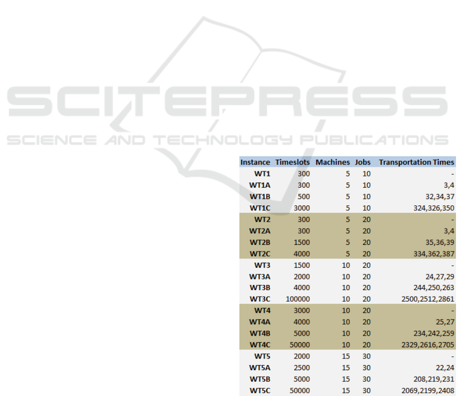
2 FJSSTT PROBLEM INSTANCES

As benchmark instances for ﬂexible job shop schedul-

ing we use the problem instances WT1-WT5, pub-

lished in (Brandimarte, 1993). Based on these in-

stances, we generated novel FJSSTT problem in-

stances in the following way: (1) For each WT in-

stance the machines are randomly grouped into three

job shops. (2) Short/moderate/long transportation

times between the job shops were calculated. A lower

bound on the makespan for the respective problem in-

stance serves as reference time R. The transportation

times are then randomly generated from the following

intervals.

• Short transportation times (network type A):

(0.09 R, 0.11 R)

• Moderate transportation times (network type B):

(0.9 R, 1.1 R)

• Long transportation times (network type C):

(9 R, 11 R)

The transportation times between the job shops sat-

isfy the triangle inequality. Within a shop the trans-

portation times are 0. Figure 1 provides an overview

of the original instances WT1-WT5 and the generated

FJSSTT instances.

Figure 1: Problem instances.

Variable Neighbourhood Search Solving Sub-problems of a Lagrangian Flexible Scheduling Problem

235

3 MATHEMATICAL MODEL

In this section we describe a mathematical model

for the FJSSTT problem with minimisation of total

weighted tardiness as objective. Lagrangian relax-

ation is applied to the machine capacity constraints,

and the resulting Lagrangian problem is decomposed

into independent job-level sub-problems.

3.1 Problem Formulation

Our problem formulation is based on (Wang et al.,

1997). I jobs with individual due dates have to be

scheduled on M available machines. We assume

immediate availability of jobs. The set of jobs I

is {0, 1, ..., I − 1} and the set of machines M is

{0, 1, ..., M − 1}. Job i consists of J

non-preemptive

operations, with J

= {0, 1, ..., J

− 1} denoting the

set of operations for job i. The operation j of job

i is denoted as (i, j). We regard simple, chain-like

precedence constraints amongst operations belong-

ing to the same job. The set of alternative machines

for operation (i, j) is denoted as H

i j

, with machine-

speciﬁc processing times. The scheduling horizon

consists of K discrete timeslots, the set of timeslots

K is {0, 1, ..., K − 1}. The beginning time of an oper-

ation is deﬁned as the beginning of the corresponding

timeslot, and the completion time as the end of the

timeslot.

In the following we introduce further parame-

ters and decision variables used in the mathematical

model. Parameters are given with a speciﬁc problem

instance as input data, whereas the decision variables

span the solution space for the scheduling problem.

Parameters

, i ∈ I : Job due dates.

i jm

, i ∈ I , j ∈ J

, m ∈ H

i j

: Processing time of oper-

ation (i, j) on machine m.

, m ∈ M , n ∈ M : Transportation time from ma-

chine m to machine n.

, i ∈ I : Job tardiness weight.

Variables

i jmk

, i ∈ I , j ∈ J

, m ∈ M , k ∈ K : The binary vari-

able δ

i jmk

is 1, if operation (i, j) is processed on

machine m at timeslot k, and 0 otherwise.

i j

, i ∈ I , j ∈ J

: Beginning time of operation (i, j).

i j

, i ∈ I , j ∈ J

: Completion time of operation (i, j).

i j

∈ H

i j

, i ∈ I , j ∈ J

: The machine assigned to op-

eration (i, j).

, m ∈ M , k ∈ K : Lagrange multiplier for timeslot

k on machine m.

The decision variables δ

i jmk

, b

i j

and c

i j

are not inde-

pendent, the following relation holds:

i jmk

(

1 if b

i j

≤ k ≤ c

i j

0 otherwise.

(1)

The optimisation objective is the minimisation of the

weighted sum of job tardiness, the optimisation prob-

lem is then

Z = min

i j

∑

i∈I

, (2)

with

= max(0,C

− D

), (3)

where C

is the completion time for job i, i.e. C

i,J

−1

Constraints Equation (2) has to be solved subject

to a number of constraints. The machine capacity

constraints are expressed as

∑

i∈I

∑

j∈J

i jmk

≤ 1, ∀m ∈ M , ∀k ∈ K . (4)

Equation (4) states that at each timeslot a machine

cannot process more than one operation. Processing

time constraints deﬁne the relation between beginning

time and completion time of operations:

i j

= b

i j

+ P

i jm

i j

− 1, ∀i ∈ I , ∀ j ∈ J

. (5)

The precedence constraints between job operations

are

i j

≥ c

i, j−1

+ 1 + R

i, j−1

i j

, ∀i ∈ I , ∀ j ∈ J

. (6)

The term “1” in (5) and (6) occurs due to the def-

inition of operation beginning time and completion

time, respectively. The precedence constraints con-

sider transportation times R

between machines. For

operations (i, j − 1) and (i, j) equation (6) states that

the beginning time of (i, j) cannot be earlier than the

arrival time at machine m

i j

. We assume immediate

availability of transport resources to move workpieces

corresponding to jobs between machines. The trans-

portation time between machines located in different

job shops covers transport between the shops as well

as shop-internal logistics activities.

The occurrence of the term R

i, j−1

i j

in (6) renders

the constraint non-linear. This non-linearity can eas-

ily be resolved, in fact the mathematical model can

be formulated as a linear integer program, which is

outside the scope of this paper.

ICORES 2017 - 6th International Conference on Operations Research and Enterprise Systems

236

3.2 Lagrangian Relaxation

For the FJSSTT problem there are two candidate

constraint sets for relaxation: precedence constraints

and machine capacity constraints. The relaxation of

precedence constraints and decomposition into inde-

pendent machine-level sub-problems is hampered by

the structure of the precedence constraints (6), as

the term R

i, j−1

i j

couples the precedence constraints

across machines. Lagrangian relaxation of machine

capacity constraints results in the relaxed problem

(λ) = min

i j

∑

i∈I

∑

m∈M

∑

k∈K

∑

i∈I

∑

j∈J

i jmk

− 1

, (7)

where λ is the vector of Lagrange multipliers. (7) has

to be solved subject to constraints (5) and (6). For a

given pair of indices m, k the term in brackets is pos-

itive if the capacity constraint for timeslot k on ma-

chine m is violated. Z

(λ) can be reformulated as

(λ) = min

i j

∑

i∈I

∑

i∈I

∑

j∈J

i j

∑

k=b

i j

−

∑

m∈M

∑

k∈K

. (8)

The structure of Z

(λ) allows the decomposition into

independent job-level sub-problems

= min

i j

∑

j∈J

i j

∑

k=b

i j

. (9)

is a one job scheduling problem and can be charac-

terised as follows, cf. (Chen et al., 1998). A job re-

quires the completion of a set of operations, and each

operation can be performed on one of several alter-

native machines. The job operations must satisfy a

set of chain-like precedence constraints (6), consider-

ing transportation times between machines. Further-

more processing time constraints (5) have to be satis-

ﬁed. Each machine has a marginal cost for utilisation

at each timeslot within the scheduling horizon under

consideration. The scheduling problem is to deter-

mine the machine and the completion time of each

operation of the job to minimise the sum of job tardi-

ness and the total cost of using the machines to com-

plete the job, where the cost of using machine m at

time k is given as λ

With the introduction of sub-problems S

, the re-

laxed problem can be reformulated,

(λ) =

∑

i∈I

−

∑

m,k

. (10)

The Lagrangian dual problem, optimising the La-

grange multiplier values, is

= max

(λ). (11)

It can be shown that Z

(λ) is concave and piece-wise

linear, thus hill-climbing methods like sub-gradient

search can be applied to solve the dual problem. The

one job scheduling problem is not N P -hard, and it

can be exactly solved with dynamic programming,

with complexity O



∑



i j





. However, we will

see in section 5 that the efﬁciency of dynamic pro-

gramming is not good enough to cope with FJSSTT

instances with many timeslots. Thus a fast heuristic

has to be developed to solve the one job scheduling

problems. In the following section we will describe

such a heuristic approach.

4 PROBLEM SOLVING

In this section we ﬁrst describe the formulation of

the dual problem, which is followed by the sub-

problem solving heuristic Variable Neighbourhood

Search (VNS).

4.1 Dual Problem

In order to solve the Lagrangian dual problem (11)

we apply two variants of the subgradient search (SG):

standard SG, and surrogate SG. The standard SG

method requires the dual problem (and thus the sub-

problems (9)) to be fully optimised, otherwise proper

subgradient directions can not be calculated. With the

dual problem fully optimised, the dual cost Z

are a

lower bound on total weighted tardiness. In the surro-

gate SG method it is sufﬁcient to solve the dual prob-

lem approximately, and thus we can apply VNS to

solve the sub-problems.

In an SG iteration l the Lagrange multipliers are

adjusted for the next iteration according to

l+1

= λ

+ s

, (12)

with a positive, scalar step-size s

and γ

, an element

of the subgradient vector γ

∑

i∈I

∑

j∈J

∗

i jmk

− 1. (13)

∗

i jmk

denotes the optimal value for δ

i jmk

in iteration l,

resulting from solving Z

(λ) with Lagrange multipli-

ers λ

. The element γ

can be interpreted as violation

Variable Neighbourhood Search Solving Sub-problems of a Lagrangian Flexible Scheduling Problem

237

of the machine capacity constraint for machine m and

timeslot k in SG iteration l.

In the standard SG method we use a common for-

mula for the calculation of step-sizes:

= α

∗

− Z

(λ

)

, (14)

with a scalar α

, 0 < α

< 2. Z

∗

is an upper bound

on Z

and is updated if feasibility repair improves

the upper bound. The search is initialised with a pa-

rameter α

, and α

is halved after Γ iterations if no

improvement in Z

has been achieved.

The step-sizes for the surrogate SG method are

calculated according to (Bragin et al., 2014):

= β

l−1



l−1



, (15)

with the surrogate subgradient vector

. The param-

eter β

is adjusted according to

= 1 −

Ω · l

, ρ = 1 −

, (16)

with conﬁguration parameters Ω and r. The step-size

calculation is initialised with conﬁguration parame-

ter s

. With the step-size formula (15) (Bragin et al.,

2014) prove convergence of the surrogate SG method,

and they show that upon convergence the lower bound

property of dual cost is preserved.

4.2 Variable Neighbourhood Search

To solve a one job scheduling problem approximately

we propose a Variable Neighbourhood Search (VNS)

heuristics with the following neighbourhood struc-

tures. Let J denote the number of operations of the

job under consideration.

Neighbourhood Structure AM1: An operation j is

chosen at random, and a random alternative ma-

chine is assigned to j. If this move causes

the violation of precedence constraints, it is re-

jected. AM1 is conﬁgured with a distance param-

eter AM1

Dist

, denoting the number of operations

for whom alternative machines are assigned cas-

cadingly. Assigning an operation j to a different

machine implies that the duration is changed.

Neighbourhood Structure AM2: An operation j is

chosen at random, and a random alternative ma-

chine is assigned to j. The new beginning time

of j and all successive operations k > j is the re-

spective earliest feasible beginning time consider-

ing the precedence constraints, plus some small,

random slack. AM2 uses a distance parameter

AM2

Dist

Neighbourhood Structure SL: Applying SL to the

incumbent solution, a neighbour solution results

from a cascade of leftward shifts, starting with a

random operation j. Let x

be the neighbour so-

lution after shifting j, and let σ denote the avail-

able slack between operations j − 1, j. The shift

distance SL

Dist

is a random integer from the inter-

val (1, σ). If σ = 0 the move SL is rejected. Other-

wise in the next step of the cascade operation j +1

is shifted leftward, with distance SL

Dist

. Succes-

sively the operations j, j + 1, ..., J are shifted left-

ward by SL

Dist

. After each shift the cost of the

resulting neighbour solution are evaluated accord-

ing to (9). The neighbour solution with minimal

cost is the result of applying SL.

Neighbourhood Structure SR: Analogous to SL the

neighbourhood structure SR deﬁnes a cascade of

rightward shifts, with a shift distance SR

Dist

. The

cascade starts with a random operation and ends

with the ﬁrst operation.

In the shaking phase of the proposed VNS the neigh-

bourhood structure AM2 is used, with increasing val-

ues for AM2

Dist

. If no improvement is achieved, the

last shaking level is the generation of a new random

solution “in the neighbourhood” of the incumbent so-

lution. The term “neighbourhood” reﬂects the fact

that the beginning time of the ﬁrst operation in the

random solution is within a maximal distance L to the

beginning time of the ﬁrst operation in the incumbent

solution. However, this last level is a massive shak-

ing of the incumbent solution, and allows to bridge

broad valleys in the ﬁtness landscape, guiding the lo-

cal search to new areas in the search space.

In the local search phase the neighbourhood struc-

tures SL → AM1 → SR are used, in the indicated se-

quence. Figure Algorithm 1 shows the pseudocode of

the proposed VNS algorithm. The algorithm is ini-

tialised in lines 2 - 7. An initial solution is generated

at random, and conﬁguration parameters are set. The

indicated values for parameters A, B, F, L, G are exem-

plary. For a randomly generated solution, parameter

G denotes the maximal distance between two consec-

utive operations.

5 COMPUTATIONAL RESULTS

In computational experiments with the problem in-

stances outlined in ﬁgure 1 we compared the perfor-

mance of two algorithms:

1. Algorithm StDP : Standard SG solves the dual

problem, dynamic programming is used to solve

ICORES 2017 - 6th International Conference on Operations Research and Enterprise Systems

238

Algorithm 1: VNS Pseudocode.

1: Initialisation

2: x ← random solution

3: A ← 50  Number of VNS iterations

4: B ← 50  Number of local search iterations

5: F ← 3  The maximal value of AM 2

Dist

6: L ← 50

7: G ← 5

8: VNS iterations

9: for a ← 1, A do

10: f ← 1

11: while f ≤ F + 1 do  Shaking loop

12: if f = F + 1 then

13:

x ← random solution “in the neighbourhood” of x

14: else

15: AM2

Dist

← f

16:

x ← AM2neighbour solution with incumbent solutionx

17: end if

18: for b ← 1, B do  Local search iterations

19: for l ← 1, 3 do

20: if l = 1 then

21: x

← SL neighbour solution with incumbent solution

22: else if l = 2 then

23: AM1

Dist

= 1

24: x

← AM1 neighbour solution with incumbent solution

25: else if l = 3 then

26: x

← SR neighbour solution with incumbent solution

27: end if

28: if cost(x

) ≤ cost(

x) then

29:

x ← x

30: end if

31: end for

32: end for

33: if cost(

x) < cost(x) then

34: x ←

35: f ← 1

36: else

37: f ← f +1

38: end if

39: end while

40: end forreturn x

the sub-problems. SG conﬁguration: α

= 2, Γ =

20.

2. Algorithm SuVNS : Surrogate SG solves the dual

problem, VNS solves the sub-problems. SG con-

ﬁguration: s

= 0.2, Ω = 25, r = 0.1.

Both algorithms use a list scheduling algorithm

for feasibility repair. Our implementation supports

concurrent computing with respect to solving sub-

problems. The experiments were performed on the

following computer hardware: Intel



Core

i7-6700

CPU @ 3.40GHz, 4 cores and 8 GB ram. On the

software side, the operating system was Microsoft



Windows

10 Pro using Java 1.8 as programming

and execution environment.

Figure 2 shows the results of computational experi-

ments with 800 SG iterations, and feasibility repair

every 2 iterations. The deterministic algorithm StDP

was executed once per problem instance. To gather

statistical results for the non-deterministic algorithm

SuVNS, 10 runs were performed with SuVNS per

problem instance. In ﬁgure 2 column UB

∗

refers to

Variable Neighbourhood Search Solving Sub-problems of a Lagrangian Flexible Scheduling Problem

239

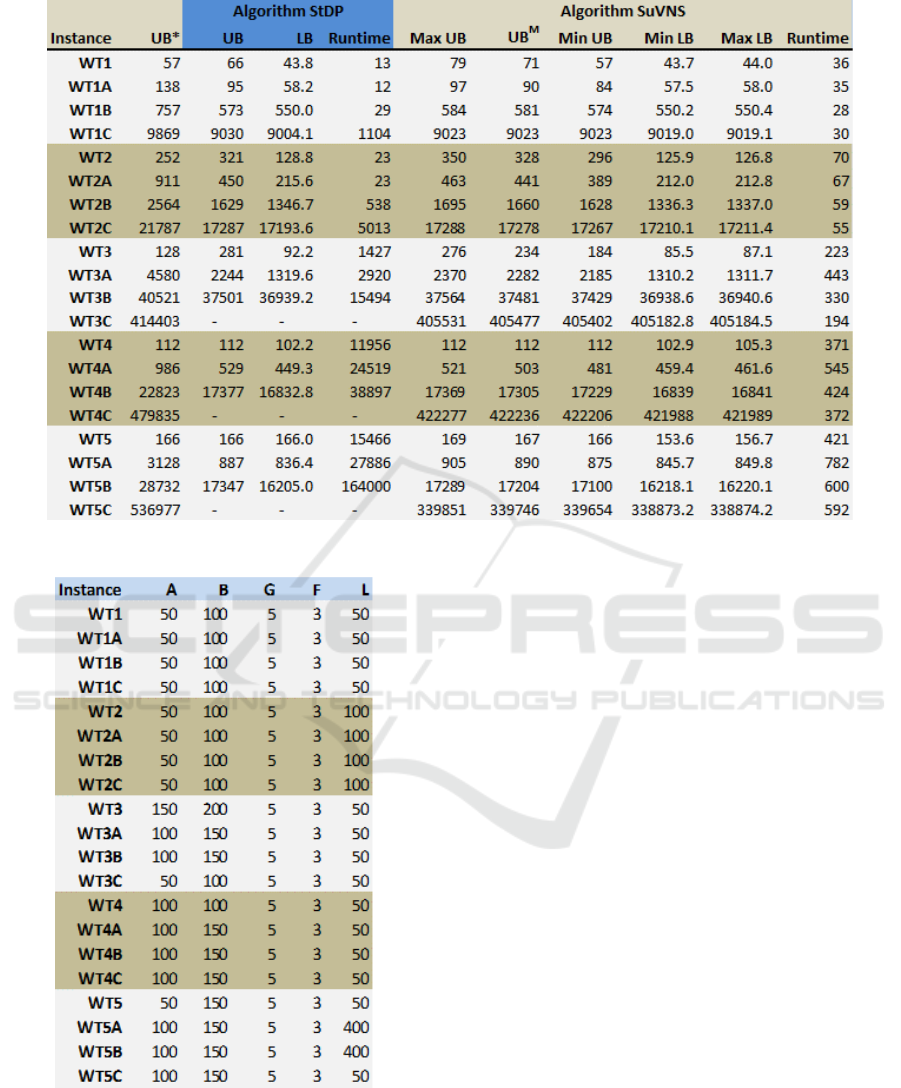
Figure 2: Computational results.

Figure 3: VNS conﬁgurations.

the best known value for total weighted tardiness for

the respective problem instance. For the instances

WT1-5 these values are taken from (Sobeyko and

onch, 2015), for the FJSSTT instances they are

calculated with list scheduling. For algorithm StDP

lower and upper bound on total weighted tardiness

are indicated (columns LB,UB) as well as the runtime

in seconds. The columns Max UB,UB

, Min U B in-

dicate maximum, mean value and minimum for total

weighted tardiness calculated with algorithm SuVNS.

Minimium and maximum for lower bounds are given

in columns Min LB, Max LB. The VNS algorithm is

conﬁgured according to ﬁgure 3. The conﬁgurations

were determined in computational experiments with

sub-problems, benchmarking VNS with exact solu-

tions calculated with dynamic programming.

Analysing the results for problem instances WT1-

5, we note that the duality gap for instances indicates

if algorithms StDP and SuVNS work well on the in-

stance. The duality gaps for WT4 and WT5 are small,

and the algorithms provide upper bounds very close

or equal to the best known values. For WT2 and WT3

the duality gaps are distinct, and the calculated up-

per bounds signiﬁcantly deviate from the best known

values. A remarkable result is provided by StDP for

WT5: the duality gap is 0, proving optimality of the

upper bound 166.

The results for the FJSSTT instances show a

strong dependence of the StDP runtime on the num-

ber of timeslots speciﬁed for the problem instance, cf.

ﬁgure 1. For WT3C, WT4C and WT5C we were not

able to calculate solutions with StDP and reasonable

runtime. The algorithm SuVNS is clearly advanta-

geous in terms of runtime, and the upper bounds are

of good quality, comparing them with StDP results.

ICORES 2017 - 6th International Conference on Operations Research and Enterprise Systems

240

6 CONCLUSIONS

The computational experiments have shown promis-

ing results. However, the list scheduling method em-

ployed for feasibility repair is rather weak, and we ex-

pect a more sophisticated heuristic to improve the re-

sults. Furthermore, it is advisable to extend the com-

putational experiments to more problem instances.

So far we have been concerned with static

scheduling problems. In a dynamic scheduling prob-

lem, a schedule is executed and disturbances like

transportation delays or machine failures hamper the

scheduled processing of operations. It would be in-

teresting to apply the proposed, distributed algorithm

to dynamic scheduling problems, and to explore the

possibilities of localised disturbance handling.

As a next step we want to improve the quality of

the feasibility repair mechanism. Also more experi-

ments with MK problems will take place. The algo-

rithm will be extended to allow dynamic rescheduling

(e.g. in case of a machine break down).

ACKNOWLEDGEMENTS

This research is funded by the Austrian Min-

istry for Transport, Innovation and Technology

www.bmvit.gv.at through the project NGMPPS-DPC.

REFERENCES

Baptiste, P., Flamini, M., and Sourd, F. (2008). Lagrangian

bounds for just-in-time job-shop scheduling. Comput-

ers & Operations Research, 35(3):906–915.

Bragin, M. A., Luh, P. B., Yan, J. H., Yu, N., and Stern,

G. A. (2014). Convergence of the Surrogate La-

grangian Relaxation Method. Journal of Optimization

Theory and Applications, 164(1):173–201.

Brandimarte, P. (1993). Routing and scheduling in a ﬂex-

ible job shop by tabu search. Annals of Operations

research, 41(3):157–183.

Buil, R., Piera, M. A., and Luh, P. B. (2012). Improve-

ment of lagrangian relaxation convergence for produc-

tion scheduling. Automation Science and Engineer-

ing, IEEE Transactions on, 9(1):137–147.

Chen, H., Chu, C., and Proth, J.-M. (1998). An im-

provement of the Lagrangean relaxation approach

for job shop scheduling: a dynamic programming

method. Robotics and Automation, IEEE Transactions

on, 14(5):786–795.

Chen, H. and Luh, P. B. (2003). An alternative frame-

work to Lagrangian relaxation approach for job shop

scheduling. European Journal of Operational Re-

search, 149(3):499–512.

Hoitomt, D. J., Luh, P. B., and Pattipati, K. R. (1993).

A practical approach to job-shop scheduling prob-

lems. Robotics and Automation, IEEE Transactions

on, 9(1):1–13.

Kaskavelis, C. A. and Caramanis, M. C. (1998). Efﬁ-

cient Lagrangian relaxation algorithms for industry

size job-shop scheduling problems. IIE transactions,

30(11):1085–1097.

Sobeyko, O. and M

onch, L. (2015). Heuristic Ap-

proaches for Scheduling Jobs in Large-scale Flexible

Job Shops. Computers & Operations Research. ac-

cepted for publication.

Wang, J., Luh, P. B., Zhao, X., and Wang, J. (1997). An

optimization-based algorithm for job shop scheduling.

Sadhana, 22(2):241–256.

Variable Neighbourhood Search Solving Sub-problems of a Lagrangian Flexible Scheduling Problem

241