
Real-time Stereo Vision System at Tunnel
Yuquan Xu
1
, Seiichi Mita
1
, Hossein Tehrani
2
and Kazuhisa Ishimaru
3
1
Research Center for Smart Vehicles, Toyota Technological Institute, 2-12-1 Hisakata, Tempaku, Nagoya, Japan
2
Driving Assist & Safety Eng. Div. 1, DENSO Corporation, 1-1, Showa cho, Kariya, Japan
3
Research & Development Dept. 2, Nippon Soken Inc., Nishio, Aichi, Japan
Keywords:
Stereo Vision, Image Deblurring, Optical Flow, Cepstrum.
Abstract:
Although stereo vision has made great progress in recent years, there are limited works which estimate the
disparity for challenging scenes such as tunnel scenes. In such scenes, owing to the low light conditions and
fast camera movement, the images are severely degraded by motion blur. These degraded images limit the
performance of the standard stereo vision algorithms. To address this issue, in this paper, we combine the
stereo vision with the image deblurring algorithms to improve the disparity result. The proposed algorithm
consists of three phases: the PSF estimation phase; the image restoration phase; and the stereo vision phase.
In the PSF estimation phase, we introduce three methods to estimate the blur kernel, which are optical flow
based algorithm, cepstrum base algorithm and simple constant kernel algorithm, respectively. In the image
restoration phase, we propose a fast non-blind image deblurring algorithm to recover the latent image. In the
last phase, we propose a multi-scale multi-path Viterbi algorithm to compute the disparity given the deblurred
images. The advantages of the proposed algorithm are demonstrated by the experiments with data sequences
acquired in the tunnel.
1 INTRODUCTION
In recent years, significant attention has been paid
to the development of autonomous vehicles and ad-
vanced driver assistance systems (ADAS). Stereo vi-
sion is an important research problem for ADAS ap-
plications and has received a great deal of attention
over the past decade. However, there is little work
considering the stereo vision in some challenge envi-
ronments, such as tunnels or low lightening condition.
For the ADAS applications, the stereo camera
pair, mounted on the vehicle, is used to estimate
the environment’s depth information from images ac-
quired by the stereo pair. However, in certain environ-
ments, such as the tunnel, the low illumination and
the fast camera movement, result in the blurring of
the stereo pair images. The blurry images reduce the
quality of stereo’s depth estimation. The motion blur
is caused by the relative movement between the cam-
era and the object during the camera’s exposure time.
The blur can be attributed to three tunnel-specific fac-
tors in ADAS applications. 1) The speed of the car,
which is typically very high, since there are no traffic
lights or sharp turns in the tunnel. 2) The distance be-
tween the camera and the object. The tunnel area is
very limited and the walls and roof of the tunnel are
near to the vehicle. 3) The length of exposure time,
which is high to account for the low illumination of
the tunnel. Stereo vision can be viewed as a matching
problem and for blurry scenes there may be multiple
matching pixels across the left and right image pair.
This phenomenon violates the basic assumption of the
stereo vision framework. Fig. 1 shows the compari-
son results of a tunnel example using the proposed
algorithm and other state-of-the-art real-time stereo
vision algorithms, Semi-Global Block-Matching Al-
gorithm (SGM) (Hirschm
¨
uller, 2008) and Multi-paths
Viterbi (MPV) (Long et al., 2014b). In Fig. 1, we
can see that the input image is highly blurred espe-
cially on the left wall, and the previous stereo vision
approaches can not reliably estimate the disparity for
such images. However, the proposed algorithm can
produce high quality disparity results, even for the
challenging scenes.
A straight forward approach to address this issue
involves the deblurring of the degraded input stereo
pairs to improve the disparity results. Motion deblur-
ring is an important research problem in low-level vi-
sion research. There are two research sub-problems
that are addressed in this research. The first problem
involves the estimation of the Point Spread Function
402
Xu Y., Mita S., Tehrani H. and Ishimaru K.
Real-time Stereo Vision System at Tunnel.
DOI: 10.5220/0006112304020409
In Proceedings of the 12th International Joint Conference on Computer Vision, Imaging and Computer Graphics Theory and Applications (VISIGRAPP 2017), pages 402-409
ISBN: 978-989-758-227-1
Copyright
c
2017 by SCITEPRESS – Science and Technology Publications, Lda. All rights reserved
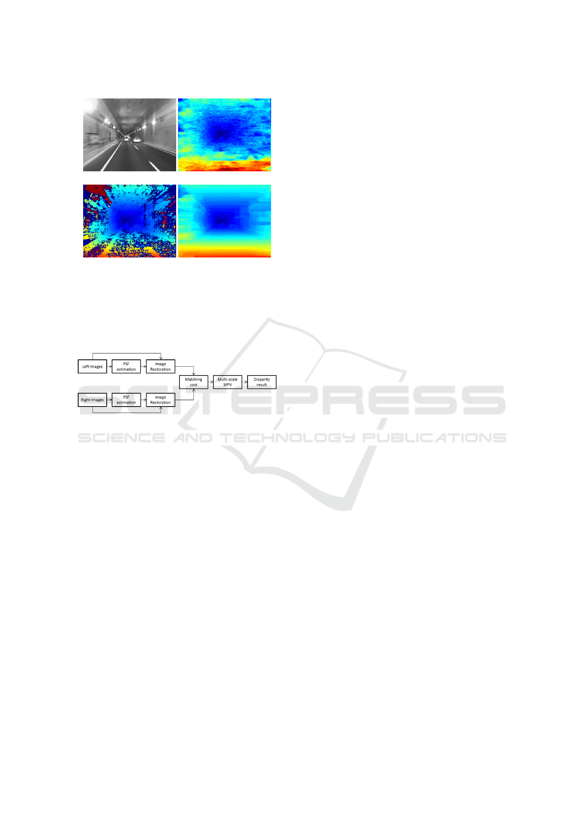
(a) (b)
(c) (d)
Figure 1: Visual comparison of our method to SGM
(Hirschm
¨
uller, 2008) and MPV (Long et al., 2014b) on an
example captured in the tunnel. (a) is the left image of
the stereo pair. (b) MPV (Long et al., 2014b). (c) SGM
(Hirschm
¨
uller, 2008). (d) The proposed method. In the dis-
parity map, red represents near objects and blue represents
distant objects.
Figure 2: The flowchart of the proposed algorithm.
(PSF) or so-called blur kernel which represents the
degradation process. The second problem involves
the recovery of the unknown latent image. Typi-
cally, most of the existing deblurring methods (Cho
and Lee, 2009; Xu and Jia, 2010) aim to deal with
the spatial-invariant blurs which are modeled as a de-
convolution problem. However, in the tunnel case,
the blur is spatially-variant. Furthermore, for ADAS
applications, the deblurring and disparity estimation
should be performed in real-time, that means the run-
ning time should be lower than 100ms. However,
other deblurring algorithms usually cost minutes to
deblur one image, which is unacceptable for real-time
application.
In this article, we introduce a real-time algorithm
to deal with the tunnel stereo vision problem. The
proposed algorithm consists of three phases, i.e., PSF
estimation phase, image restoration phase and stereo
vision phase. In the PSF estimation phase, the tradi-
tional iteration based framework’s computational cost
is reduced by utilizing three different algorithms to
directly estimate the spatially-variant blur kernel by
using optical flow, cepstrum and a simple constant
kernel. After we estimate the PSF of the image, a fast
non-blind image deblurring algorithm is introduced to
remove the blur effect of the images. Last we propose
a multi-scale MPV algorithm to compute the disparity
result. Our proposed approach is real-time which is
significantly important for practical applications. We
show the flowchart of the proposed algorithm in Fig.
2
2 RELATED WORK
Stereo vision is one of the basic problems in com-
puter vision and has made tremendous progress in
last decades. Scharstein and Szeliski (Scharstein and
Szeliski, 2002) introduced a categorization scheme
for stereo algorithms, which classified the various
stereo algorithms into two classes including local and
global methods. Local algorithms usually contain
four steps: (1) matching cost computation; (2) cost
aggregation; (3) disparity computation; (4) the op-
tional post processing. The matching cost compu-
tation methods include standard window-based algo-
rithms, normalized cross correlation (NCC), Census
Transform algorithm (Zabih and Woodfill, 1994), and
recently CNN based cost (Zbontar and LeCun, 2014).
The cost aggregation algorithms contain unnormal-
ized box filtering, bilateral filter and guided image fil-
ter (He et al., 2013). On the other hand, the global
methods make explicit smoothness assumptions and
then solve an optimization problem from the match-
ing cost and omit the cost aggregation step. The op-
timization algorithms include dynamic programming
(Veksler, 2005), belief propagation (Sun et al., 2003),
Viterbi (Long et al., 2014a; Long et al., 2014b) and
graph cuts (Boykov et al., 2001). SGM (Hirschm
¨
uller,
2008) is a hybrid of local and global method that ex-
pands the single-directional 1D scanline optimization
process to multidirectional 1D scan-line optimization.
Removing the blur effects of the images is a well-
studied problem. For spatial-invariant blind image
deblurring issue, Fergus et al. (Fergus et al., 2006)
firstly proposed a successful variational Bayesian
framework to estimate the complex motion blur ker-
nel. In (Cho and Lee, 2009), a fast deblurring method
was proposed by introducing a prediction step. The
similar step was used in (Xu and Jia, 2010) (Xu et al.,
2012). For spatial-variant blur issue, Joshi et al.
(Joshi et al., 2010) introduced inertial measurement
sensors to record the motion path of the camera to
recover the latent image. Then the projective motion-
blur model was introduced by (Tai et al., 2011) and
used in (Whyte et al., 2011) (Hirsch et al., 2011).
Zheng et al. (Zheng et al., 2013) proposed a forward
motion model which is more relevant to our work, but
Real-time Stereo Vision System at Tunnel
403

(a) (b)
Figure 3: (a) is the blurry input, (b) is the blur kernel in each
local area of the image.
their work is too time-consuming for practical appli-
cation. We refer the readers to the (Wang and Tao,
2014) for the recent progress of the image deblurring.
3 STEREO VISION ALGORITHM
In this section, we introduce a coarse-to-fine frame-
work to estimate the disparity result based on the de-
blurred images. We adopt the structural similarity
(SSIM) to measure the matching cost between left and
right deblur images.In this coarse-to-fine framework,
we generate the 3 layers Gaussian pyramid of the de-
blurred images, and each coarser layer is half size of
the finer layer. Then we utilize the MPV (Long et al.,
2014a) method to estimate the disparity result from
the coarsest to the finest layer. The cost function of
proposed algorithm is:
E(D) = E
D
(D) +E
TV
(D) (1)
Where D represents the disparity result, E
D
(D)
represents the SSIM cost of deblurring images and
E
TV
(D) represents the TV constraints of disparity.
Figure 4: Viterbi path to find optimum disparity.
The problem of stereo matching can be modeled
as finding the disparity map D that minimizes the en-
ergy function E(D). In this case, the Viterbi algorithm
can be used to search the optimum solution (Son and
Seiichi, 2006). We build a graph to represent the dis-
parities of the image pixels along one line, where each
node in this graph represents a disparity assigned to a
pixel and each edge represents a candidate disparity
change between two pixels in the same path. Viterbi
algorithm operates on individual rows and find the op-
timum ”path” of nodes through disparity space from
one side of the image to the other as shown in Fig 4.
To find the optimum disparity value, we solve follow-
ing cost function:
d
t
= arg min
d
V (t −1,d
t−1
) + SSIM(t, d)+ λ|d − d
t−1
|
(2)
where d
t
represents the disparity at pixel t, V (t −
1,d
t−1
) represents the energy of a node with pixel t −
1 with disparity d
t−1
, SSIM(t,d) represents the SSIM
cost with pixel t and disparity d and λ|d −d
t−1
| is the
smoothing penalty term.
To increase the robustness of the Viterbi algo-
rithm, four bi-directional (horizontal, vertical, and 2
diagonals) Viterbi paths are used to provide good cov-
erage of the 2D image. The flowchart of the Multi-
path Viterbi algorithm is shown in Fig. 5.
With the results on the coarser layer, we only con-
sider a small candidate disparity range. This multi-
scale MPV algorithm is much faster than (Long et al.,
2014a) and more stable to get better results on some
textureless area.
Figure 5: The flowchart of the Multi-path Viterbi algorithm.
4 PSF ESTIMATION
In this section, we estimate the motion kernel of the
tunnel images. For a given image with long exposure
time, the estimating the motion blur kernels are not
trivial. Fortunately in the tunnel case, the exposure
times are limited by the frame rate. Additionally, the
vehicle typically travels in a straight path in the tun-
nel. Therefore, the motion observed during the expo-
sure will be relatively smooth and the PSF in a small
local area can be approximated as the linear kernel, as
VISAPP 2017 - International Conference on Computer Vision Theory and Applications
404
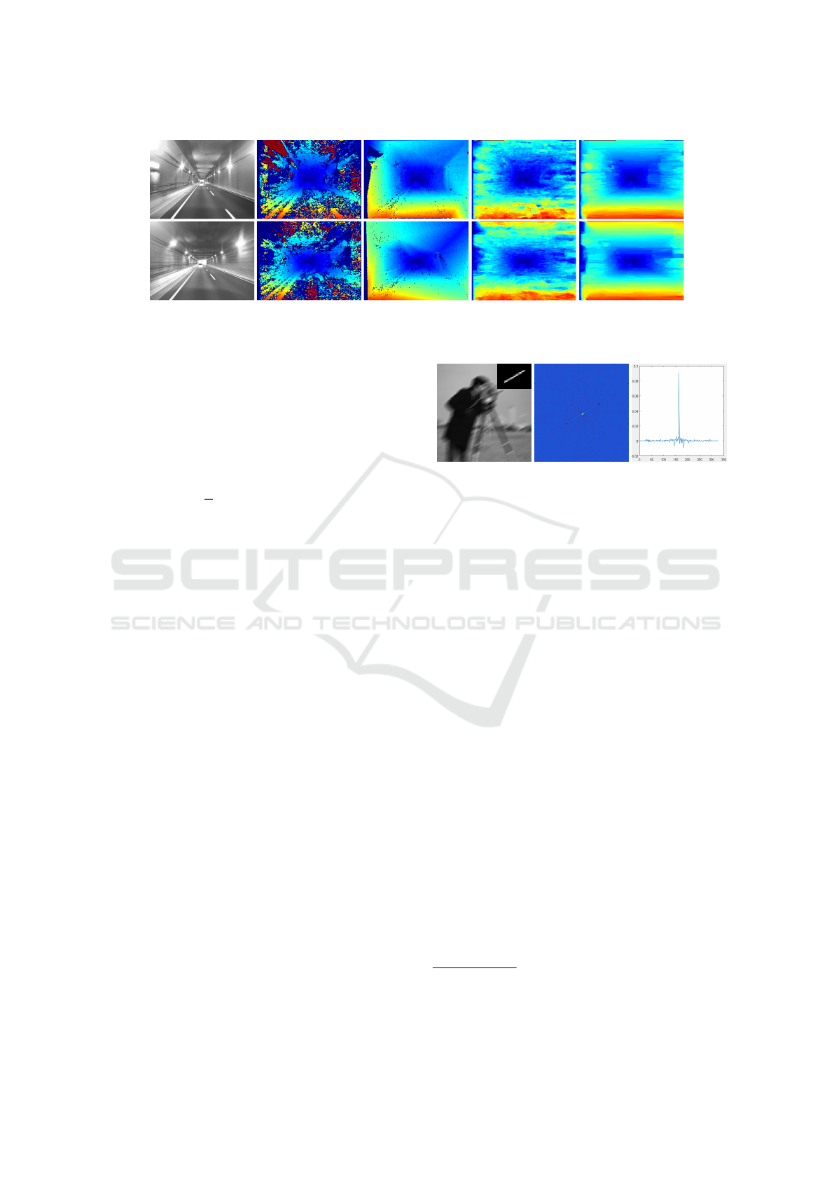
Figure 6: The first column is the original image. The second to last column are the disparity results of SGM (Hirschm
¨
uller,
2008), ELAS (Geiger et al., 2011), MPV (Long et al., 2014b) and the proposed method respectively.
shown in Fig. 3. This approximation helps in the case
of the spatially-varying blur since estimating an arbi-
trary kernel for each individual pixel would be pro-
hibitively expensive. Based on this assumption, the
blur kernel at each pixel is a straight line which is de-
termined by two parameters, i.e., the length and the
angle. Then the blurry input can be formulated as:
b =
1
Z
∑
i
[(ω
i
∗ l) ⊗ f
i
] + n (3)
where b is the blurry input, ω
i
is the window func-
tion to select a sub-region of the image, l is the latent
image we want to recover, i is the index of the sub-
region, ∗ denotes the element-wise multiplication, ⊗
denotes the convolution process, Z is normalization
factor of the window function, n is the additive noise,
f
i
represents the blur kernel of the i −th sub-region of
the image, respectively. For the PSF, we have:
f (x, y) =
1/L others
0 y = x tan θ, 0 ≤ x ≤ L cos θ
(4)
where x and y are pixel index and L is the length of the
kernel, θ is the angle of the kernel, respectively. Then
we introduce three algorithms to estimate this kind of
blur kernel for the blurry input.
4.1 Optical Flow
Since the motion blur is caused by the relative motion
of the camera and objects, it follows that the knowl-
edge of the actual camera motion between consecu-
tive image pairs that can provide significant informa-
tion when performing image deblurring. We assume
that the camera moves nearly along a straight line be-
tween two successive frames and the optical flow of
these two frames can represent the blur kernel for the
blurry input. To compute the optical flow, we have the
cost function as Equ. (5)
E(w) = E
D
(w) + λE
S
(w) (5)
(a) (b) (c)
Figure 7: (a) is the blurry image and the blur kernel in its
right up. (b) is the cepstrum of blurry input. (c) is the value
alone the blur angle in the cepstrum.
where w is the flow vector, λ is the smoothing param-
eter, E
D
(w) is the data term and E
S
(w) is smoothing
term, respectively. For E
D
(w) and E
S
(w) we have:
E
D
(w) =
k
I
2
(u + w) − I
1
(w)
k
2
+
α
k
∇I
2
(u + w) − ∇I
1
(w)
k
2
(6)
E
S
(w) =
|
∇w
|
(7)
where I
1
and I
2
are two successive frames, ∇ =
(∂
x
,∂
y
) represents the gradient of the image, α ∈ [0,1]
denotes a linear weight. The smoothing term is the
Total Variation (TV) constraint. We use the Suc-
cessive Over-Relaxation (SOR) method to solve Equ.
(5). Since the input image is blurry and we actually
don’t need the optical flow for every pixel of the im-
age
1
, we downsample the input left and right image
to 1/4 size which can not only reduce the blurry effect
in the image but also reduce the computation time of
the algorithm. Then we upsample the optical flow to
represent the blur kernel of the image.
4.2 Cepstrum
To deblur the image, we first segment the blurry in-
put into several overlapped patches and assume that
in each sub-region the blur kernel is a straight line.
1
Actually we deblur the input image block by block, so
we only need an optical flow for every small local area of
the input, not every pixel
Real-time Stereo Vision System at Tunnel
405

Based on this assumption, we can compute the cep-
strum of the image to identify the angle and length of
this kind of linear kernel. The cepstrum of an image
is defined as (Rom, 1975):
C(g) = F
−1
(log(|F(g)|) (8)
where F and F
−1
denote the Fourier transform and
inverse Fourier transform , C(g) is the cepstrum of
the image g. In practice, the cepstrum of the image is
usually expressed as:
C(g) = F
−1
(log(|F(g)| + 1) (9)
This linear degrade process for each sub-patch is
described as Equ. (10)
s
b
= s
l
⊗ f + n (10)
where s
b
and s
l
denote the sub-patch of the blurred
and clear image.
In the case of ignoring the additive noise n, we can
formulate Equ. (10) to cepstrum domain as:
C(s
b
) = C(s
l
) +C( f ) (11)
where C(s
b
), C(s
l
) and C( f ) represent the cepstrum
of blurred image s
b
, s
l
and f . Therefore the cepstrum
of blurred image is modeled as the sum of the cep-
strum of the clear image and the cepstrum of a blur
kernel, which means the convolution operation be-
comes additive in cepstrum domain, thus the blur is
easy to detect.
Fig. 7 shows an example of how we use the cep-
strum to detect the blur kernel of the image. Fig. 7
(a) shows a blurry and noisy image. The blur ker-
nel has 20 pixels length and 30-degree angle and the
variance of the Gaussian noise is 0.03. We show the
cepstrum of the blurry input in Fig. 7 (b), in which we
can clearly see a straight line along the 30-degree. In
practice, we adopt the Radon transform to detect this
angle as the blur angle and then we rotate the cep-
strum to make this line to be horizontal. Fig. 7 (c)
shows the values on this line of the cepstrum and we
can see two negative peaks in this line. We compute
the distance between these two negative peaks and the
blur length is half of the distance. Finally, we can es-
timate the angle and length of the blur kernel. For a
blurry tunnel input, we segment it to some overlapped
cloacal areas and use the cepstrum to estimate the blur
kernel of this sub-region.
4.3 Proposed Method
In autonomous vehicle applications, the stereo vision
algorithm is required to generate the disparities in
real-time continuously and stably. Although we have
Table 1: Computation time.
Methods Time Environment
Optical flow 9.8s Intel i7 4790 CPU
Cepstrum 7.8s Intel i7 4790 CPU
Proposed 1.4s Intel i7 4790 CPU
Proposed 96ms GTX TITAN X GPU
proposed two algorithms to estimate the blur kernel,
the computational time is not real-time or less than
100ms. Therefore, we further reduce the computa-
tional complexity of the deblurring process for the
stereo pairs. More specifically, we adopt a constant
kernel as an approximate motion kernel for all the
pixels of the tunnel images as shown in Fig. 8 (d).
In this constant kernel, we pre-define a point in the
image to represent the vanishing point along the trav-
eling direction of the vehicle and the angle of the blur
kernel in each subregion can be determined by the
vector from the vanishing point to the central point.
The length of the kernel is determined by the vehi-
cle speed and the shutter speed, and we can read from
the camera and the vehicle CAN. In Fig. 8, we can
see that using this simple kernel the disparity result
is similar for the optical flow and cepstrum methods.
We also compare the computation time of these three
algorithms including the image restoration and stereo
vision phase in Table 1 and size of the input stereo
image is 640 × 480.
5 NON-BLIND DEBLURRING
ALGORITHM
After we get the PSF estimation, we define the fol-
lowing cost function to restore the clear image:
E(l) = ||b −
1
Z
∑
i
(ω
i
∗ l) ⊗ f
i
||
2
+ γ|∇l| (12)
where γ denotes the smoothing parameter.
In practice, we divide the input blurry input into
several overlapping parts and in each part we deblur
the image by solving Eq. 13
E(s
l
) = ||s
b
− s
l
⊗ f
i
||
2
+ γ|∇s
l
| (13)
We utilize the half-quadratic penalty method (Kr-
ishnan and Fergus, 2009) to recover each sub-region.
We introduce two auxiliary variables u
x
and u
y
, and
iterated solving following function:
s
l
= F
−1
γ
(
F(∂
x
)∗F(u
x
)+F(∂
y
)∗F(u
y
)
)
+F( f )∗F(s
b
)
γ
(
|F(∂
x
)|
2
+|F(∂
y
)|
2
)
+|F( f )|
2
u
x
= argmin
u
x
γ|u
x
| + (u
x
− ∂
x
s
l
)
2
u
y
= argmin
u
y
γ|u
y
| + (u
y
− ∂
y
s
l
)
2
(14)
VISAPP 2017 - International Conference on Computer Vision Theory and Applications
406
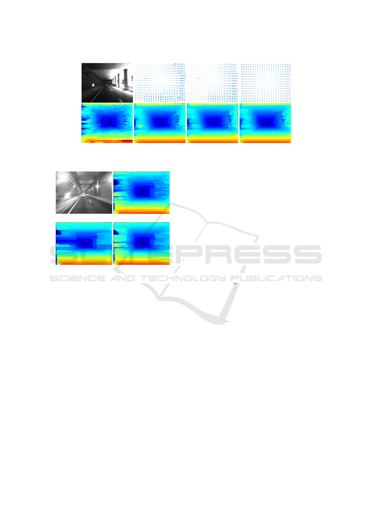
Figure 8: The first column is the original image and the disparity result of MPV (Long et al., 2014b). The second to last
column are the PSF and disparity results of optical flow, cepstrum and the proposed kernel methods, respectively.
(a) (b)
(c) (d)
Figure 9: (a) is the blurry and noisy left image. (b) is the
stereo result without noise reduction. (c) is the stereo result
using the denoise algorithm as pre-processing method. (d)
is the stereo result of the proposed method.
After all the sub-regions are restored, we obtain
a weighted sum of these sub-regions with Hanning
window function to produce the final results. Since
in the proposed method the blur kernel is not totally
correct in some area, the γ for the proposed method
is 10 times bigger than the optical flow and cepstrum
methods.
5.1 Noisy Case
In the low light condition such as a tunnel, the cap-
tured images are not only blurry but also contain high-
level noise. Simply using the denoising algorithm
as a pre-processing step will improve the quality the
deblurred result, but significant artifacts can be ob-
servable along the deblurred image edges and/or the
image structure may be over-smoothed (Tai and Lin,
2012).
Since in our simple case our blur kernel is not cor-
rect in some parts, we already use a large smoothing
parameter to compensate the result. Using the denois-
ing algorithm will further make the final result even
more smooth. In this paper, we adopt the follow-
ing strategy to handle this problem as shown in Alg.
1. First, we denoise the input image using fast non-
local means algorithm (Goossens et al., 2010). With
the denoising output
e
b we compute a deblurring re-
sult
e
l. Then, we refine
e
b according to the motion blur
constraints from
e
l avoid over-sharpening and/or over-
smoothing in the denoised image. Last, we use pre-
vious non-blind algorithm to deblur the refined
e
b and
get the deblurred image. Specifically, we compute the
e
l by minimizing following cost function:
E(
e
l) = ||b −
1
Z
∑
i
(ω
i
∗
e
l) ⊗ f
i
||
2
+ λ
1
||∇l||
2
(15)
After we get
e
l, we refine the blurry image
e
b as:
E(
e
b) = ||
e
b −
1
Z
∑
i
(ω
i
∗
e
l) ⊗ f
i
||
2
+ λ
2
||∇
e
b||
2
+ λ
3
||b −
e
b||
2
(16)
Since Equation 15 and 16 are both l2 norm func-
tion, we can directly compute the closed-form solu-
tion using FFT. In Fig. 9, we show the stereo results
of this noise reduction method. In Fig. 9 (b), we can
see that the stereo result without dealing the noise still
contains noise. In Fig. 9 (c), the non-local means al-
gorithm is adopted to be a pre-processing step and the
stereo result is over-smoothed. In Fig. 9 (d), our re-
sult is relatively better than others with less noises and
correct disparity results for blurry and noisy areas.
6 EXPERIMENT
We evaluated the proposed method on the experimen-
tal autonomous car with the stereo camera mounted
Real-time Stereo Vision System at Tunnel
407
Algorithm 1: Framework for denoising and deblurring.
1: Input: The noisy and blurry image b
2: Output: The denoised and deblurred image l
3: Compute denoised image
e
b by (Goossens et al.,
2010)
4: Solve
e
l by minimize Equation 15.
5: Refine
e
b by minimize Equation 16.
6: Solve l by minimize Equation 12.
Table 2: Result on the tunnel scene.
Stereo Out-Noc(3px) Avg-Noc
Proposed 12.21% 2.12px
SGM (Hirschm
¨
uller, 2008) 32.97% 4.77px
ELAS (Geiger et al., 2011) 20.10% 3.52px
MPV (Long et al., 2014b) 24.33% 4.19px
outside the car and the stereo camera is Bumblebee
BBX3-13S2C-38. We construct a tunnel stereo vision
dataset that contain 200 examples using the Velodyne
HDL-32E 3D laser scanner (10 Hz, 32 laser beams,
range: 100 m) to get precise distance and construct
the ground truth data. We compare the quantitative
values of the proposed algorithm and other real-time
methods in Table 2 and the proposed algorithm out-
performs other existing methods for the tunnel im-
ages. We show some of the qualitative results in Fig.
6.
After computing the disparity, we validate the pro-
posed algorithm within a ADAS application. We
compute the road surface by using the disparity re-
sults. The road surface is detected by using the his-
togram of disparity in horizontal and vertical direc-
tion. We denote the V-disparity (H
v
) to be the row-
based histogram of the different disparities in each
row of the disparity map and the U-disparity (H
u
) to
be the column-based histogram. Then we use the V-
disparity and U-disparity (Long et al., 2014a) Viterbi
based optimization method to detect the road surface.
The results are shown in Fig. 10. We can see the dis-
parity results of SGM (Hirschm
¨
uller, 2008) contain
much more holes and errors in the road surface, and
generate a slightly more irregular road area and road
boundary.
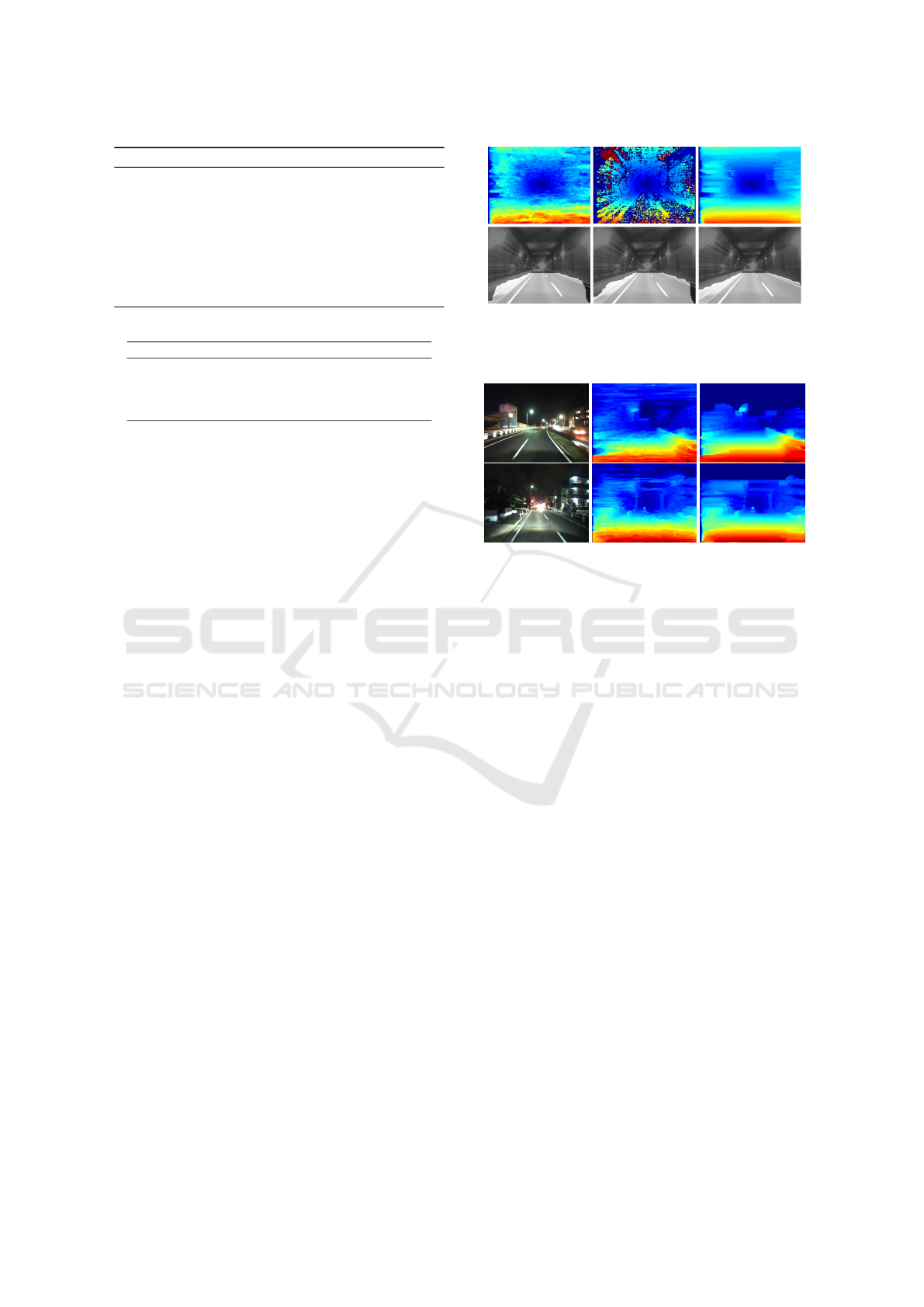
6.1 Extend to Non-tunnel Case
We evaluate the proposed algorithm on some non-
tunnel images in low light conditions such as night-
time, the captured images will also be blurred and
noisy. Although the background of the nighttime im-
ages are more complicated than the tunnel case and
the blur kernel of the proposed method is not suit-
able in some parts of the image, the proposed algo-
rithm still can significantly improve the stereo results
Figure 10: Road surface comparison. The first to last
columns represent the disparity result and corresponding
road surface estimation of method (Long et al., 2014b),
(Hirschm
¨
uller, 2008) and the propose simple method.
Figure 11: Results on the nighttime images. The first to last
columns represent is the input left image of stereo pair, the
stereo results of (Long et al., 2014b) and our results.
as shown in Fig. 11.
7 CONCLUSION
In this paper, we have presented a novel algorithm to
improve stereo vision in the tunnel. Typically, the mo-
tion kernel for tunnel cases is spatially-variant and
difficult to be estimated in the real-time. Consid-
ering the characteristics of the tunnel case, we seg-
ment the image into overlapped subregions and as-
sume the motion kernel in each region to be a lin-
ear function. Then we utilize three algorithms to es-
timate the PSF by optical flow, cepstrum and simple
constant kernel. We compare the results of these three
approaches and find that the proposed simple kernel is
enough to produce promising disparity results with re-
duced computational efficiency. This simple method
together with the fast non-blind deblurring algorithm
and multi-scale MPV method are the final real-time
deblurring-stereo framework for the tunnel case. The
experiment results show the proposed algorithm can
effectively and efficiently deal with the real tunnel im-
ages. Furthermore although the proposed algorithm is
designed for tunnel images, it performs well on other
images captured at low light conditions.
VISAPP 2017 - International Conference on Computer Vision Theory and Applications
408

REFERENCES
Boykov, Y., Veksler, O., and Zabih, R. (2001). Fast ap-
proximate energy minimization via graph cuts. Pat-
tern Analysis and Machine Intelligence, IEEE Trans-
actions on, 23(11):1222–1239.
Cho, S. and Lee, S. (2009). Fast motion deblurring. In
ACM Transactions on Graphics (TOG), volume 28,
page 145. ACM.
Fergus, R., Singh, B., Hertzmann, A., Roweis, S. T., and
Freeman, W. T. (2006). Removing camera shake from
a single photograph. In ACM Transactions on Graph-
ics (TOG), volume 25, pages 787–794. ACM.
Geiger, A., Roser, M., and Urtasun, R. (2011). Efficient
large-scale stereo matching. In Computer Vision–
ACCV 2010, pages 25–38. Springer.
Goossens, B., Luong, H., Aelterman, J., Pi
ˇ
zurica, A.,
and Philips, W. (2010). A gpu-accelerated real-
time nlmeans algorithm for denoising color video se-
quences. In International Conference on Advanced
Concepts for Intelligent Vision Systems, pages 46–57.
Springer.
He, K., Sun, J., and Tang, X. (2013). Guided image filter-
ing. Pattern Analysis and Machine Intelligence, IEEE
Transactions on, 35(6):1397–1409.
Hirsch, M., Schuler, C. J., Harmeling, S., and Scholkopf, B.
(2011). Fast removal of non-uniform camera shake.
In Computer Vision (ICCV), 2011 IEEE International
Conference on, pages 463–470. IEEE.
Hirschm
¨
uller, H. (2008). Stereo processing by semiglobal
matching and mutual information. Pattern Analy-
sis and Machine Intelligence, IEEE Transactions on,
30(2):328–341.
Joshi, N., Kang, S. B., Zitnick, C. L., and Szeliski, R.
(2010). Image deblurring using inertial measure-
ment sensors. ACM Transactions on Graphics (TOG),
29(4):30.
Krishnan, D. and Fergus, R. (2009). Fast image deconvo-
lution using hyper-laplacian priors. In Advances in
Neural Information Processing Systems, pages 1033–
1041.
Long, Q., Xie, Q., Mita, S., Ishimaru, K., and Shirai, N.
(2014a). A real-time dense stereo matching method
for critical environment sensing in autonomous driv-
ing. In Intelligent Transportation Systems (ITSC),
2014 IEEE 17th International Conference on, pages
853–860. IEEE.
Long, Q., Xie, Q., Mita, S., Tehrani, H., Ishimaru, K., and
Guo, C. (2014b). Real-time dense disparity estima-
tion based on multi-path viterbi for intelligent vehicle
applications. In Proceedings of the British Machine
Vision Conference. BMVA Press.
Rom, R. (1975). On the cepstrum of two-dimensional func-
tions (corresp.). Information Theory, IEEE Transac-
tions on, 21(2):214–217.
Scharstein, D. and Szeliski, R. (2002). A taxonomy and
evaluation of dense two-frame stereo correspondence
algorithms. International journal of computer vision,
47(1-3):7–42.
Son, T. T. and Seiichi, M. (2006). Stereo matching algo-
rithm using a simplified trellis diagram iteratively and
bi-directionally. IEICE transactions on information
and systems, 89(1):314–325.
Sun, J., Zheng, N.-N., and Shum, H.-Y. (2003). Stereo
matching using belief propagation. Pattern Analy-
sis and Machine Intelligence, IEEE Transactions on,
25(7):787–800.
Tai, Y.-W. and Lin, S. (2012). Motion-aware noise filtering
for deblurring of noisy and blurry images. In Com-
puter Vision and Pattern Recognition (CVPR), 2012
IEEE Conference on, pages 17–24. IEEE.
Tai, Y.-W., Tan, P., and Brown, M. S. (2011). Richardson-
lucy deblurring for scenes under a projective mo-
tion path. Pattern Analysis and Machine Intelligence,
IEEE Transactions on, 33(8):1603–1618.
Veksler, O. (2005). Stereo correspondence by dynamic pro-
gramming on a tree. In Computer Vision and Pattern
Recognition, 2005. CVPR 2005. IEEE Computer So-
ciety Conference on, volume 2, pages 384–390. IEEE.
Wang, R. and Tao, D. (2014). Recent progress in image
deblurring. arXiv preprint arXiv:1409.6838.
Whyte, O., Sivic, J., and Zisserman, A. (2011). Deblurring
shaken and partially saturated images. In Computer
Vision Workshops (ICCV Workshops), 2011 IEEE In-
ternational Conference on, pages 745–752. IEEE.
Xu, L. and Jia, J. (2010). Two-phase kernel estimation for
robust motion deblurring. In Computer Vision–ECCV
2010, pages 157–170. Springer.
Xu, Y., Hu, X., Wang, L., and Peng, S. (2012). Single im-
age blind deblurring with image decomposition. In
Acoustics, Speech and Signal Processing (ICASSP),
2012 IEEE International Conference on, pages 929–
932. IEEE.
Zabih, R. and Woodfill, J. (1994). Non-parametric local
transforms for computing visual correspondence. In
Computer VisionłECCV’94, pages 151–158. Springer.
Zbontar, J. and LeCun, Y. (2014). Computing the stereo
matching cost with a convolutional neural network.
arXiv preprint arXiv:1409.4326.
Zheng, S., Xu, L., and Jia, J. (2013). Forward motion de-
blurring. In Proceedings of the IEEE International
Conference on Computer Vision, pages 1465–1472.
Real-time Stereo Vision System at Tunnel
409
