
3D Plane Labeling Stereo Matching with Content Aware Adaptive
Windows
Luis Horna and Robert B. Fisher
IPAB, The University of Edinburgh, Edinburgh, U.K.
Keywords:
Stereo Matching, 3D Labeling, Adaptive Windows.
Abstract:
In this paper, we present an algorithm that exploits both the underlying 3D structure and image entropy to
generate an adaptive matching window. The presented algorithm estimates real valued disparity maps by
smartly exploring a 3D search space using a novel hypothesis generation approach that acts like a propagation
scheduler. The proposed approach is among the top performing results when evaluated in the Middlebury,
KITTI 2015 benchmarks.
1 INTRODUCTION
The problem of 3D plane labeling to estimate depth
from two or more images has become the focus area
of modern stereo matching algorithms. The core is-
sue in 3D plane labeling using two images (left I
l
and
right I
r
views of a scene) is finding the correspon-
dences for each pixel from image I
l
to I
r
by assigning
a 3D plane that produces a real valued disparity
1
. This
process is better modeled as an optimization problem
where the objective is to compute the disparity assign-
ment that minimizes eq.1.
E(D) = argmin
D
NumP
∑
p
{C
p
(D
p
) +
∑
q∈N(p)
V
pq
(D
p
,D
q
)}
(1)
E(D) is the cost of the disparity assignment (en-
ergy), D is a set of planes and D
p
encodes a plane
at pixel p, that gives the disparity of the pixel at p
with respect to another image. D
p
(q) is the disparity
estimated using plane D
p
evaluated at pixel q. The
plane D
p
has two parameters: a 3D unit normal vec-
tor ˆn
p
= (n
x
p
,n
y
p
,n
z
p
) and disparity d
p
. The disparity
of pixel q = (x
q
,y
q
) using D
p
is given by:
D
p
(q) = a ∗ x
q
+ b ∗ y
q
+ c (2)
where a = − ˆn
x
p
/ ˆn
z
p
, b = −ˆn
y
p
/ ˆn
z
p
and c = ( ˆn
x
p
∗x
q
+
ˆn
y
p
∗ y
q
+ ˆn
z
p
∗ d
p
)/ ˆn
z
p
as in (Bleyer et al., 2011). C
p
is a function that measures the similarity/dissimilarity
1
The displacement along a search area is known as dis-
parity.
of two pixels (e.g. I
l
(p) and I
r
(p + D
p
(p))), and
NumP is the number of pixels in the image. N(p)
is a neighborhood around p, and q is a neighbor of
p. V
pq
(smoothness term) is a function that evalu-
ates how well the disparity at position p fits its neigh-
bors. Eq.1 is typically represented as Markov Ran-
dom Field (MRF) and minimized using either Graph
Cuts (GC), Loopy Belief Propagation (LBP) or Tree
Re-weighted with Sequential (T RW-S) update. In this
paper inference/minimization is done using T RW -
S(Kolmogorov, 2007).
In this paper, we present an algorithm that exploits
the underlying 3D structure, image texture to gener-
ate an adaptive matching window, and a 3D search
using a novel hypothesis generation approach to esti-
mate real valued disparity maps.
2 RELATED WORK
The idea of assigning planes per pixel to estimate
sub-pixel disparity has been previously used in (Klaus
et al., 2006; Woodford et al., 2007; Bleyer et al., 2011;
Besse et al., 2012; Olsson et al., 2013; Heise et al.,
2013; Taniai et al., 2014; Sinha et al., 2014; Yam-
aguchi et al., 2014). These algorithms can be clas-
sified in two categories: fixed plane inference (FPI)
and dynamic plane inference (DPI). FPI algorithms
make an initial disparity estimation and then extract
the planes, which are then used during the inference
process to estimate disparity. By contrast DPI algo-
rithms assign one or more planes to each pixel, and
then propagate “good” planes (i.e. low/high scores
162
Horna L. and B. Fisher R.
3D Plane Labeling Stereo Matching with Content Aware Adaptive Windows.
DOI: 10.5220/0006105401620171
In Proceedings of the 12th International Joint Conference on Computer Vision, Imaging and Computer Graphics Theory and Applications (VISIGRAPP 2017), pages 162-171
ISBN: 978-989-758-227-1
Copyright
c
2017 by SCITEPRESS – Science and Technology Publications, Lda. All rights reserved

depending on the cost function) to neighbors/regions
under the assumption that neighbors/regions are likely
to have the same plane. Then in a refinement stage the
planes are improved, thus the planes are dynamically
updated. DPI algorithms in particular have become
the state of the art (e.g. (Bleyer et al., 2011; Besse
et al., 2012; Heise et al., 2013; Taniai et al., 2014)).
Common issues in DPI algorithms include the use
of large adaptive windows (commonly using (Yoon
and Kweon, 2006)) or segment (Li et al., 2015) based
similarity cost to compute the similarity/dissimilarity
cost, which can result in a strong bias towards large
planes. A possible solution to this issue is to change
the window size, which requires either some assump-
tion about the 3D structure or image content. How-
ever, changing the window size can result in poor per-
formance in textureless areas and thus requires addi-
tional assumptions such as the uniqueness constraint
or occlusion penalties. Another issue in DPI algo-
rithms such as (Bleyer et al., 2011; Besse et al., 2012)
is that the hypothesis generation and propagation is
done sequentially.
2.1 Contributions
To address some of the issues described the proposed
approach makes the following contributions:
• Content aware adaptive window aggregation: Re-
duces error and loss of details.
• Use of a cost function that imposes a local hy-
pothesis uniqueness, unlike (Klaus et al., 2006;
Woodford et al., 2007; Olsson et al., 2013; Ya-
maguchi et al., 2014; Sinha et al., 2014; Bleyer
et al., 2011; Besse et al., 2012; Taniai et al., 2014):
Helps to handle textureless surfaces, and does not
required higher order interactions (unlike (Vogel
et al., 2015)) in a MRF.
• Use of a cost function that penalizes disparity val-
ues outside a defined search range: Prevents in-
valid disparity values assignment.
• Use of a single global hypothesis per disparity
plane: Eliminates the need to update multiple hy-
potheses.
• Use of a hypothesis generator that acts as a prop-
agation scheduler: Helps to do a search in a 3D
space.
3 PROPOSED ALGORITHM
The proposed approach to estimate a 3D plane label-
ing per pixel has the following components:
• Content aware slanted windows to compute the
data term (pixel similarity measure).
• Uniqueness and out of range terms.
• Adaptive search range.
• Smoothness term that adapts to image content.
• Hypothesis generation/update that acts as a prop-
agation scheduler.
The novel content aware windows exploit both in-
tensity and 3D structure (if available) to adapt the
window size and similarity function. It’s important to
note that the proposed hypothesis generation provides
an alternative to sequential algorithms (e.g. (Bleyer
et al., 2011; Besse et al., 2012)) and does not impose
restrictions to the pairwise interactions like (Taniai
et al., 2014).
3.1 Content Aware Adaptive Similarity
Function
DPI algorithms commonly use the adaptive window
(eq.4) from (Yoon and Kweon, 2006), which has the
following issues: bias towards large planes (good
quality in textureless areas), center pixel bias for
large windows (results in loss of detail, e.g. fig.1),
and noisy results for small windows. The center
pixel bias can be reduced by using the windows from
(Zhang et al., 2009), which adapts better to local im-
age changes, but can give poor results if the windows
are poorly estimated or window size is not large (par-
ticularly in textureless areas). To compensate for the
center pixel bias while keeping good performance in
textureless areas, a texture measure L
p
(eq.3) is used
to balance the influence of eq.4 and eq.5 (fixed size
modified version of (Zhang et al., 2009)) in eq.7.
L
p
=
(
e
−
T
p
τ
w
T
p
=
1
Z
∑
q∈N(p)
e
−
|I
p
−I
q
|
σ
r
h(p)
)
(3)
AW
p
(D
p
) =
1
Z
∑
q∈N(p)
e
−
|I
p
−I
q
|
σ
r
c
q
(D
p
) (4)
CW
p
(D
p
) =
1
Z
v
∑
q∈N
v
(p)
e
−
|I
p
−I
q
|
σ
r
CW
h
q
(D
p
) (5)
CW
h
q
(D
p
) =
1
Z
h
∑
s∈N
h
(q)
e
−
|I
s
−I
q
|
σ
r
c
s
(D
p
) (6)
C
p
(D
p
) = L
p
· AW
p
(D
p
) + (1 − L
p
) ·CW
p
(D
p
) (7)
where Z, Z
h
, Z
v
are normalization constants such that
the weights in the neighbourhood add up to one, h(p)
is a 5 × 5 entropy filter, |I
p
− I
q
| is the L1 distance in
RGB space, N(p) is the neighborhood around p (n×n
window), N
h
(p) and N
v
(q) are the horizontal (1 × n)
and vertical (n × 1) neighborhoods around p and q.
Eq.3 is the adaptively filtered version of h(p), which
is done to clean the noisy measure, and better balance
AW
p
and CW
p
close to edges.
3D Plane Labeling Stereo Matching with Content Aware Adaptive Windows
163
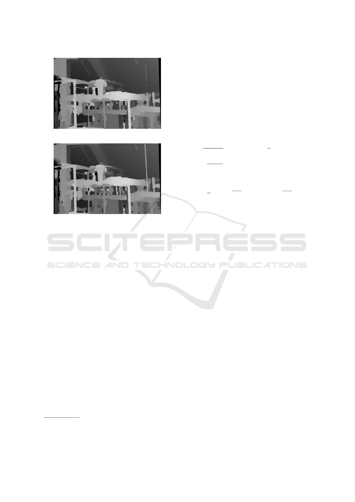
(a)
(b)
Figure 1: Raw result of Pipes image with AW (a) and AW +
CW (b) functions. Parameters used as in sec.6.
The adaptive window from (Zhang et al., 2009)
was modified as follows: Use of range terms for ver-
tical and horizontal directions. Only horizontal arms
are computed, while the vertical arm remains of a
fixed size. The pixel similarity function is given by:
c
p
(D
p
) = αc
1
p
(D
p
(p)) + c
2
p
(D
p
(p)) (8)
c
1
p
(D
p
) = min(|∇I
1
p
− ∇I
2
p+D
p
|,τ
grad
) (9)
c
2
p
(D
p
) = min(χ(I
1
,I
2
, p,D
p
),τ
cen
) (10)
where, I
1
is the reference image, and I
2
is the
target image, c
1
p
(D
p
) is the truncated absolute differ-
ences of gradients, c
2
p
(D
p
) is the Truncated Hamming
distance of census transform(Zabih and Li, 1994)), χ
computes the census transform at p and displacement
D
p
and Hamming distance, α balances the pixel-wise
cost influence. Note that D
p
(p) is the disparity result-
ing from the evaluation of plane D
p
at pixel p.
The adaptive window described so far works un-
der the assumption that the window size remains con-
stant all over the image, which can lead to either loss
of detail
2
(large windows), noisy results (small win-
dows), and bias towards large planes. To reduce these
effects the window size is selected based on a local
2
In particular adaptive windows have a tendency to lose
thin vertical details.
measure W
p
, which describes the behavior of an ini-
tial disparity map gradient around a region. A region
is a superpixel segment obtained using SLIC(Achanta
et al., 2012). The behavior of the initial disparity
map gradient is first measured along the pixels in the
segment perimeter (eq.11), then a segment difference
measure is computed using the median disparity of
neighbouring segments (eq.12), and later propagated
per pixel (eq.13) to reduce the effect of noise from the
initial disparity map. Thus window size at each pixel
p is computed using n = Ω(p) in eq.14.
ˆw
p
=
1
K
w
|
ˆ
N(p)|
∑
q∈
ˆ
N(p)
|
˜
d
p
−
˜
d
q
| ≥
2
5
K
w
(11)
w
p
=
(
1
K
w
|
ˆ
N(p)|
∑
q∈
ˆ
N(p)
min(|
˜
d
p
−
˜
d
q
|,K
w
) : ˆw
p
> τ
0
w
0 : otherwise
(12)
W
p
=
(
1
Z
∑
q∈N(p)
e
−
|I
p
−I
q
|
σ
r
w
p
Z =
∑
q∈N(p)
e
−
|I
p
−I
q
|
σ
r
)
(13)
Ω(p) =
(
ω
1
: W
p
> τ
nn
and T
p
> τ
h
ω
2
: otherwise
(14)
where,
˜
d
p
and
˜
d
q
are the median disparities (to
compensate for noise in the initial estimate) of the
segments where pixels p and q come from.
ˆ
N(p) is
the perimeter of the segment where p comes from.
Notice that eq.12 computes a value per segment,
while eq.13 does it per pixel by aggregating neighbor-
ing values based on intensity similarity. τ
nn
is dynam-
ically computed from W
p
using Otsu threshold. Eq.11
measures the number of pixels that can be considered
and edge for being above a threshold.
3.2 Uniqueness and Out of Range
Terms
The Similarity function described above only takes
into consideration intensity to compute a matching
score. However, this has the implicit assumption that
each pixel has a unique match, which in general is not
necessarily true (e.g.2), especially in occluded areas
and textureless regions that are prone to have multi-
ple matches (see red boxes in fig.3). Eq.15 penalizes
each pixel that has multiple matches (similar to (Kol-
mogorov and Zabih, 2001)).
U(D
p
) =
(
τ
unique
: L(Dp)
0 : otherwise
(15)
where L(Dp) is true when a pixel p is mapped to
d + D
p
which has more than one match. This is done
VISAPP 2017 - International Conference on Computer Vision Theory and Applications
164

per hypotheses, which means it’s a local uniqueness
terms, unlike (Kolmogorov and Zabih, 2001) and (Vo-
gel et al., 2015) where it’s represented as part of the
MRF.
Figure 2: Example of uniqueness constraint violation; two
pixels (red arrows) in left image scanline map to a single
pixel in right image (red pixel).
A plane D
p
evaluated at a different pixel q in
the image could have disparity values that lie outside
a defined search range of disparities. Eq.16 penal-
izes disparity values that lie outside a defined search
range.
O(D
p
) =
1 − exp(−|D
p
− minD|/σ
d
) : D
p
< minD
1 − exp(−|D
p
− maxD|/σ
d
) : D
p
> maxD
0 : otherwise
(16)
where minD and maxD are the minimum and max-
imum of the disparity search range, while σ
d
is the
maximum deviation allowed for values outside the
search range. Eq.7 is updated to include eq.15 and
eq.16, which then becomes:
ˆ
C
p
(D
p
) = C
p
(D
p
) +U (D
p
) + O(D
p
) (17)
Note that the proposed uniqueness term requires
to keep track of its current value after inference to up-
date the current cost (eq.17) and prevent energy from
oscillating in later iterations.
3.3 Search Range Detection
To detect spurious disparities the probability distri-
bution (from the normalized disparity histogram) of
each disparity present in both the left and right dis-
parity maps is computed using an initial search range
[minD,maxD], and an n-point (n is 18% of the initial
disparity search range) Parzen window is applied to
smooth the probability distribution.
Finally, a search finds the lowest (min
ˆ
D) and
largest disparities (max
ˆ
D) that are above a threshold
τ
maxD
and τ
minD
=
2
3
τ
maxD
. It’s possible that min
ˆ
D
is over estimated and max
ˆ
D under estimated, which
is addressed by min
ˆ
D = max(minD, min
ˆ
D − ∆minD),
and max
ˆ
D = min(maxD, max
ˆ
D + ∆maxD). The esti-
mated bounds on the disparities are used to eliminate
or penalize unrealistic disparities. max
ˆ
D is used dur-
ing the inference process, and min
ˆ
D during the post-
processing stage.
3.4 Smoothness Term
The assumption made by the proposed edge model is
that possible depth discontinuities are allowed small
variations, while areas with a similar intensity are al-
lowed to have larger changes, by contrast in (Besse
et al., 2012; Taniai et al., 2014) the maximum varia-
tion is constant.
V
pq
(D
p
,D
q
) =
(
w
pq
λω(D
p
,D
q
,K2) : |F
p
− F
q
| < τ
di f f
w
pq
λω(D
p
,D
q
,K1) : otherwise
(18)
w
pq
=
(
1
Z
n
e
−|I
ms
(p)−I
ms
(q)|
Z
n
=
∑
q∈N(p)
e
−|I
ms
(p)−I
ms
(q)|
)
(19)
where K1 < K2, I
ms
is a gray level image after
applying the quick shift segmentation
3
(Vedaldi and
Soatto, 2008; Vedaldi and Fulkerson, 2008), w
pq
and
λ are weights, F
p
and F
q
come from a local cue map
F, and τ
di f f
is a threshold, which means the growth
limit of the smoothness term adapts based on the local
cue map F (eq.22), while ω(D
p
,D
q
,K) is given by:
ω(D
p
,D
q
,K) = min(|D
p
(p)−D
q
(p)|+|D
q
(q)−D
p
(q)|,K)
(20)
F
p
is computed using the intensity gradient of the
reference image, and is used to locate possible depth
discontinuities. Using the image gradient can lead to
problems in areas where the gradient is noisy (e.g. im-
age or texture is noisy). This issue can be partially
addressed by filtering both the image and gradient,
which can provide a two-fold advantage. First, the
gray level of the reference image is filtered (eq.21) to
remove potential sources of noise (e.g. noisy edges or
sensor noise). Second, a filter is applied to the gra-
dient magnitude (eq.22) to remove false edges (e.g.
small letters on a wall).
ˆ
I
g
(p) =
(
1
Z
∑
q∈N(p)
e
−
|I
p
−I
q
|
σ
r
|∇I
g
(p)|
Z =
∑
q∈N(p)
e
−
|I
p
−I
q
|
σ
r
)
(21)
F
p
=
(
1
Z
∑
q∈N(p)
e
−
|I
p
−I
q
|
σ
r
|∇
ˆ
I
g
(p)|
Z =
∑
q∈N(p)
e
−
|I
p
−I
q
|
σ
r
)
(22)
where I is the color image, |∇
ˆ
I
g
(q)| = |∇
x
ˆ
I
g
(q)| +
|∇
y
ˆ
I
g
(q)|, and ∇
x
ˆ
I
g
(q) and ∇
y
ˆ
I
g
(q) are obtained us-
ing the Sobel gradient operator.
3
To handle noise in the image.
3D Plane Labeling Stereo Matching with Content Aware Adaptive Windows
165

(a) (b) (c)
Figure 3: Raw result of Teddy image (τ
grad
= 5/255, τ
cen
= 5/25, random initialization, and no multi-scale). (a) Groundtruth
Teddy image; (b) Uniqueness term is disabled; (c) Uniqueness term is enabled.
4 HYPOTHESIS GENERATION
AND PROPAGATION
The model described so far makes the assumption that
each pixel has associated a set of planes from which
a single optimal plane assignment (D) is found us-
ing T RW -S. The proposed hypothesis generation al-
gorithm will give each pixel p a set GH
p
= D
p
∪H
p
∪
DS
p
∪ V
p
. D
p
is the current solution, H
p
is gener-
ated from pixel coordinates using (r-sampling), DS
p
is generated from the pixels that belong to the same
segment
4
(P-sampling), V
p
is generated from pixels
coming from another view (V -sampling). Using these
disparity planes at each pixel allows the following:
1. Pixels can keep their current plane assignment D
p
.
2. Pixels propagate their planes to close and distant
pixels via r-sampling.
3. Segments help to propagate large disparity planes
to distant pixels via P-sampling.
4. Views propagate their planes via V -sampling.
Note that hypothesis generation is done from a
single disparity plane assignment D for both left and
right views, and the hypothesis generation is effec-
tively acting as a propagation scheduler once infer-
ence is done.
4.1 r-sampling
Algorithms that use plane propagation commonly as-
sume that neighboring pixels are likely to have the
same plane (Bleyer et al., 2011; Besse et al., 2012)
or that planes are shared within a certain area (Taniai
et al., 2014). The proposed r-sampling tries to gen-
erate hypotheses that are shared in a region (similar
to (Taniai et al., 2014)), but also include a few planes
from a distant region. The pixel coordinates used for
4
A segment will be a set of pixels that are grouped using
some logical criteria e.g. spatial distance and color similar-
ity.
sampling are (X,Y ) =
(divs ∗ b(x + i)/divsc + r + i,
divs∗b(y+ j)/divsc+r + j) | ( j,i) ∈ [−r,r]×[−r,r]
,
which come from a window of width 2r + 1. (x , y) are
the coordinates of pixel p, and divs = 2r + 1. The r-
sampled plane at pixel p sampled with (i, j) is given
by:
ˆ
D
i j
p
= D
XY
p
(23)
This sampling is repeated for each (i, j) ∈ [−r,r]×
[−r,r] generated by a window centered at p, which
means each pixel has a set of hypotheses:
H
p
=
r
[
i=−r
r
[
j=−r
ˆ
D
i j
p
(24)
The purpose of this sampling strategy is to in-
clude the planes from all neighbors in the divs ×divs
window centered at p and also neighbors that come
from distant divs × divs windows. Fig.4 shows how a
3 × 3 window (i.e r = 1) would generate several hy-
potheses, where each colored box is a different plane.
For illustration purposes we will center our atten-
tion around the “red plane” and its eight neighbors.
H
1
...H
n
represent the hypothesis generated by using i
and j according to eq.24. In particular fig.4 demon-
strates how each of the non-purple planes are trans-
formed into a hypothesis. Also note that the planes
from the purple pixels are used as well (although they
are not necessarily the same!). This is meant to allow
the propagation of distant neighbors. This hypothesis
generation strategy is similar to that of (Taniai et al.,
2014), but ours does not impose a sub-modular re-
quirement to the pairwise interaction in the generated
hypothesis.
4.2 P-sampling
One assumption commonly used in stereo matching
is that pixels with similar intensity have a similar
disparity value or disparity plane. An easy way to
group pixels is to use super-pixels or segments (e.g.
VISAPP 2017 - International Conference on Computer Vision Theory and Applications
166

(a) (b) (c)
Figure 4: Hypothesis generation: (a) Teddy image; (b) r-sampling; (c) Ds
p
= Dφ(p).
SLIC(Achanta et al., 2012) in this paper), which are
then initialized with a plane. The disparity plane Ds
p
is assigned to a segment s
p
by randomly selecting a
plane from the planes associated with the pixels that
belong to the segment:
Ds
p
= Dφ(p) (25)
Ds
p
denotes a plane at pixel p that was assigned
by function Dφ(p) which randomly selects a plane
such that it belongs to the same segment as pixel p.
This criteria will only generate one hypothesis per
pixel, although there may be other planes in the same
segment. This is done under the assumption that one
of planes selected may be correct without the need
of fitting one plane to the entire segment. Although
each Ds
p
is assigned to several pixels (depending on
the super-pixel algorithm used), it may be desirable to
create additional hypotheses from the segments that
surround s
p
. To sample the neighboring segments the
centroid of each s
p
is computed, all neighboring s
q
centroid segments are sorted by their polar angle with
respect to s
p
, and finally only the first P elements are
selected.
DS
p
=
(
Ds
p
∪ (
P
[
i=1
Ds
qi
)
Θ(s
q1
,s
p
) < ... < Θ(s
qP
,s
p
)
)
(26)
where s
qi
∈ N(s
p
) and Θ(s
qi
,s
p
) is the function
that evaluates the polar angle with respect to the cen-
troid of s
p
.
4.3 V -sampling
The hypotheses H
p
and DS
p
so far are generated from
only one view. Since left and right sets of disparity
planes are computed it’s possible that one them con-
tains planes which could be used to generate a better
set of hypothesis. The additional set of hypotheses
is computed by mapping the planes H
p
∪ DS
p
from
the other view to the current image. This process will
be referred to as V -sampling and can be expressed by
V
p
= Dw
p
∪ Hw
p
∪ DSw
p
, where Dw
p
is the current
solution of the other view, Hw
p
and DSw
p
are the
mapped versions of r-sampling and P-sampling hy-
potheses from the other view. Note that this doubles
the number of hypotheses. For instance: assume two
views are used, then for r = 2 and P = 6 the number
of hypotheses generated would be 32 for one view,
but after doing V -sampling the number of hypotheses
would be 64. Note that (Bleyer et al., 2011) follows
a similar approach (i.e. mapping the planes from one
view to the other), but only generates one hypothesis.
5 REFINEMENT
Using the algorithms from the previous section, hy-
potheses are generated and a unique disparity plane
is assigned to each pixel (i.e D
p
). The solution is
then refined by generating a new set of hypothe-
ses Gre f
p
= D
p
∪ Hre f
p
∪ DSre f
p
with perturba-
tions(Bleyer et al., 2011) added to the plane param-
eters (normal vector ˆn
p
and disparity d
p
), and the do-
ing inference once again. The hypothesis refinement
process is:
1. Given the current disparity map D
curr
, ∆n
1
= κ,
∆d
1
= Sr ×κ as input.
2. For t = 1 to s steps do:
(a) compute pixel hypothesis re-sampling (Hre f
p
),
see sec.5.1.
(b) compute segment hypothesis re-sampling
(DSre f
p
), see sec.5.2.
(c) compute Gre f
p
= D
p
∪Hre f
p
∪DSre f
p
and ob-
tain a new solution
ˆ
D
curr
.
(d) set D
curr
=
ˆ
D
curr
, ∆n
t
= ∆n
t−1
/2 and ∆d
t
=
∆d
t−1
/2.
This means that for each pixel in the disparity map
three situations can happen: a plane is propagated
from a neighbor, a plane is refined and propagated
3D Plane Labeling Stereo Matching with Content Aware Adaptive Windows
167

from a neighbor, or a plane stays the same. Prop-
agation is done simultaneously during the hypothesis
refinement process, which happens due to the way hy-
potheses are generated. Also note that V-sampling is
not used. To the best of our knowledge no other al-
gorithm performs simultaneous propagation and re-
finement, which could have the potential to reduce
the space needed to store hypotheses. The refinement
process doubles the number of hypotheses. For in-
stance: if r-sampling (r = 2) and P-sampling(P = 6)
generate 32 hypotheses, then refinement would add
32 additional hypotheses (with perturbations added).
5.1 Pixel Hypothesis Re-sampling
To overcome local minima of the current dispar-
ity plane assignment, and obtain a refined version
of r-sampling, each pixel is updated by randomly
adding a perturbation selected from [−∆n
t
,∆n
t
] (uni-
form distribution) and [−∆d
t
,∆d
t
] (uniform distribu-
tion) which are initially set to ∆n
1
= κ (the new nor-
mal vector has to be normalized) and ∆d
1
= Sr × κ,
(Sr search range in disparity units), with κ = 0.2 as
recommended in (Besse et al., 2012). This process
is repeated several times. After each step ∆n
t
and
∆d
t
are updated by setting them to ∆n
t
= ∆n
t−1
/2
and ∆d
t
= ∆d
t−1
/2. This process generates a new set
of hypotheses Hre f
p
= H
p
∪ Hn
p
where Hn
p
is gen-
erated using r-sampling from D
p
after perturbations
have been added.
5.2 Segment Hypothesis Re-sampling
Refined versions of the disparity planes image seg-
ment are obtained by creating variants of the current
set of disparity planes per image segment. First, for
each segment in the current image random disparity
planes (DSr
p
) are generated using P-sampling and
then noise is added. This generates a new set of hy-
potheses DSu
p
= Ψ(DSr
p
∪ DSrn
p
), where DSr
p
was
generated via P-sampling, DSrn
p
is the perturbed ver-
sion of DSr
p
, and Ψ is a function that takes each
pair of planes DSr
i
p
and DSrn
i
p
and returns the one
whose cost locally minimizes eq.1, with respect to
the current solution. This leaves P plane hypotheses
per segment. Another set of hypotheses DSU
p
is then
generated, in which each segment SU
p
has a number
from [1...n]. These numbers are used as multipliers
to control the random interval [−∆d
t
,∆d
t
], such that
∆
i
d
t
= i ×∆d
t
. Thus each element of DSU
p
is the ∆
i
d
t
perturbed version of a plane generated by Dφ(p) to al-
low large jumps of disparity that can change an entire
segment. This re-sampling produces a set of hypothe-
ses DSre f
p
= DSu
p
∪ DSU
p
.
6 OVERALL DISPARITY
ESTIMATION PROCESS
The disparity estimation process can now be summa-
rized as follows:
1. Initialize solution Dle f t and Dright to either a
random plane per pixel or initialize from a pre-
computed disparity map.
2. For t = 1 to s steps do:
(a) Generate hypotheses GHle ft
p
and GHright
p
,
see sec.4.
(b) Do inference and compute new solutions
ˆ
Dle f t
and
ˆ
Dright.
(c) Refine the new solutions
ˆ
Dle f t and
ˆ
Dright, see
sec.5.
(d) set Dle f t =
ˆ
Dle f t and Dright =
ˆ
Dright.
Random initialization is done by selecting a ran-
dom uniform disparity. The normal ˆn is selected from
the uniform distribution of a unit sphere. ∆d and ∆ ˆn
are selected in the same way. Fig.5 shows interme-
diate stages for the teddy image, using the proposed
algorithm with random initialization. It can be ob-
served that our approach is effectively propagating the
planes and also minimizing eq.1. Notice that in the
first propagation the outline of the underlying 3D sur-
face can already be seen. When using a pre-computed
disparity map
5
to initialize the current solution, the
normal vectors are computed at five scales, averag-
ing, and creating a plane per pixel by estimating the
parameters of eq.2 using the normal vectors and cur-
rent disparity.
Finally, the proposed algorithm is extended to
multi-scale:
1. Precompute disparity maps Dle f t
pre
and
Dright
pre
(e.g. using SGM or random ini-
tialization).
2. Estimate window size from Dle f t
pre
and
Dright
pre
(if disparity map was precomputed).
3. Compute initial solution Dle f t and Dright by
downscaling Dle ft
pre
and Dright
pre
to one quar-
ter size and solving.
4. Compute updated solution at half-size by initial-
izing with current Dle f t and Dright.
5. Compute updated solution at full-size by combin-
ing Dle f t
pre
and Dright
pre
with current Dle f t and
Dright. i.e compute GH pre
p
∪ GH
p
for left and
right, then do inference to update current solu-
tions, and update maxD (sec.3.3).
6. Compute updated solution at full-size by initializ-
ing with current Dle f t and Dright.
5
The pre-computed disparity map is obtained using
SGM, see support material.
VISAPP 2017 - International Conference on Computer Vision Theory and Applications
168
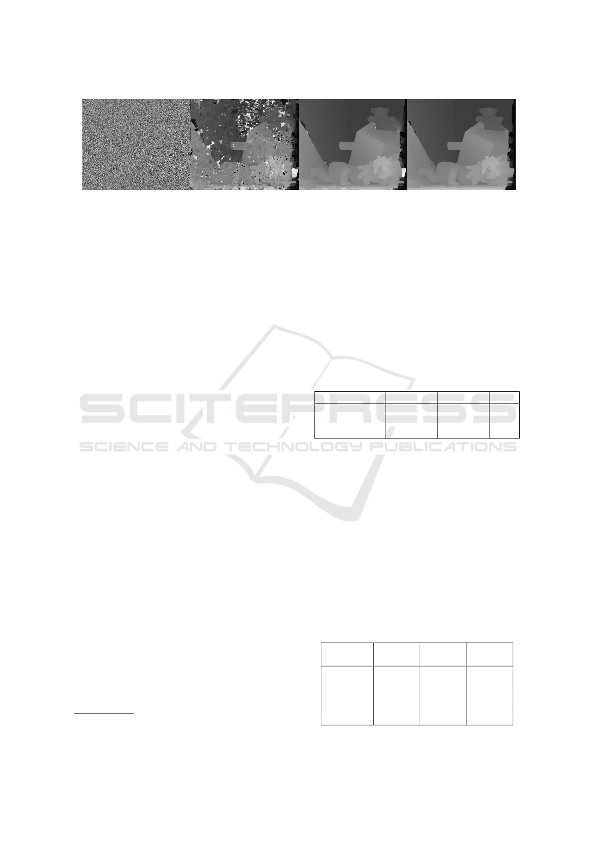
(a) (b) (c) (d)
Figure 5: Proposed algorithm with random initialization (τ
grad
= 5/255, τ
cen
= 5/25, and no multi-scale), intermediate and
final results: (a) Initial random configuration; (b) First propagation, E = 123,257.02; (c) First Refinement, E = 87,134.61;
(d) Final Result, E = 82,334.98.
7. Compute occlusion detection and post-
processing.
The post-processing is done by computing oc-
cluded, and mismatched areas as in (
ˇ
Zbontar and Le-
Cun, 2015). Then masks containing non-occluded
areas, and depth edges
6
are eroded and marked as
occluded to reduce the fattening effect. Then minD
is updated (sec.3.3), and disparities lower than minD
are marked as occluded. The occluded areas are then
filled in using simple background interpolation and
filtered by applying a weighted median filter. The
non-occluded areas are NOT post-processed.
All experimental results were carried out using
the multi-scale approach with pre-computed initial-
ization. The proposed algorithm uses the following
parameters for all scales: aggregation window sizes
of ω
1
= 41 × 41, ω
2
= 25 × 25, τ
grad
= 3/255, τ
cen
=
9/25, σ
r
= 10/255, σ
d
= 0.5, τ
w
= 2.5, τ
di f f
= 0.07,
α = 30, K
1
= 1, K
2
= 6, r = 2, P = 6, τ
h
= 2, τ
0
w
= 0.5,
K
w
= 8, τ
unique
= 0.01. For quarter and half size
λ = 0.06, and λ = 0.12 for full size. The disparity
estimation is iterated 4 times at quarter size, 1 time
at half-size and 4 times at full size. The refinement
iterations are set to 5 times each scale. These param-
eters were obtained by using the Middlebury train-
ing data, and every fifth image from KITTI 2015 and
2012 training data.
7 PROPOSED APPROACH VS.
STATE OF THE ART
The approach presented in this paper was validated
in three stages. First, the proposed content aware
adaptive windows are compared to the traditional ap-
proach, as well as the tolerance to noise and evalua-
tion of r−sampling performance. Then the proposed
algorithm is extensively validated on three data sets:
6
detected using Canny edge detector.
The new Middlebury (15 images) data set (Scharstein
et al., 2014), KITTI 2015(Menze and Geiger, 2015)
and 2012(Geiger et al., 2012) (up to 200 images).
The only parameters that are set differently are ∆minD
(10 for Middlebury and 5 for KITTI), ∆maxD (60 for
Middlebury and 20 for KITTI) and τ
maxD
(0.0028 for
Middlebury and 0.0003 for KITTI).
Table 1: Comparative table of the proposed content aware
function vs adaptive windows. Evaluation done with the
Middlebury training data set at half size in non occluded
areas before post-processing.
Function %bad noc avg. error rms
AW 13.62 2.00 7.62
AW +CW 13.58 1.98 7.67
AW +CW +U 12.95 1.82 7.28
To test the performance of the proposed similar-
ity function three competing functions are compared
(tab.1): AW is the traditional approach (eq.4) with
the enabled out of range term , but no uniqueness
term. AW + CW is the proposed adaptive window
(eq.7) with the enabled out of range term, but no
uniqueness term. AW +CW +U is the proposed adap-
tive window with the out of range and local unique-
ness terms (eq.17). Our innovations (eq.17) clearly
improve on the popular adaptive windows(Yoon and
Kweon, 2006) commonly used in DPI algorithms.
Table 2: Evaluation of r-sampling and proposed approach
(all stages enabled) tolerance to noise in initial disparity
map, using every fifth image from KITTI 2015 training
data. ns0 no noise, and added disparity noise [−1, 1] (ns1),
[−2,2] (ns2), [−3, 3] (ns3).
Algorithm
%bad
D1-bg
%bad
D1-fg
%bad
D1-all
ns0
2.96 9.26 3.86
LSL
2.90 9.55 3.86
ns1
2.94 9.49 3.89
ns2
2.96 9.39 3.88
ns3
2.94 9.85 3.94
3D Plane Labeling Stereo Matching with Content Aware Adaptive Windows
169

To evaluate the effectiveness of r-sampling we re-
place it with the pixel shared hypotheses LSL from
(Taniai et al., 2014). In tab.2 our sampling strategy
(ns0) in general matches the performance of LSL, and
even gives improved performance for foreground ob-
jects D1 − f g, which is caused by the larger number
of hypotheses 25 for r-sampling vs. 16 for L SL due
to different hypothesis generation strategies. The per-
formance of our approach in tab.2 shows that the pro-
posed approach ns0 is robust to several levels of uni-
form real valued noise added to the initial disparity
map.
The main competitors to our algorithm are
MCNCC(
ˇ
Zbontar and LeCun, 2015) and MDP(Li
et al., 2016a), since they were evaluated using the
same data sets (see tab.3 and tab.4). To compare to the
state of the art, from all data sets competitors were se-
lected by choosing the best performing convolutional
neural network algorithms and the best performing al-
gorithm not using convolutional neural networks. For
the KITTI 2015 and 2012 results, algorithms must ap-
pear in both data sets evaluation tables. The proposed
algorithm is among top performers in the Middle-
bury (tab.3) and KITTI 2015/2012 (tab.4 and tab.5).
In tab.3 the disparity map is evaluated only in non-
occluded areas, integer and sub-pixel scores are com-
puted using an error pixel threshold of 2.0 (rank 9
th
out of 44) and 0.5 (rank 8
th
out of 44) respectively.
Table 3: Comparative table of results (on non-occluded pix-
els) on the new Middlebury data set. Only non-anonymous
entries are used for comparison: PMSC(Li et al., 2016b),
Mesh and MeshE(Zhang et al., 2015), APAP(Park and
Yoon, 2016), MCNCC(
ˇ
Zbontar and LeCun, 2015), MDP(Li
et al., 2016a).
Algorithm
%bad >
2.0
%bad >
0.5
avg.
error
rms
Our
7
10.50
9th
43.2
8th
3.17 15.6
PMSC
8
6.87
1st
39.1
1st
2.27 12.9
MeshE
9
7.29
2nd
40.1
2nd
2.50 15.4
APAP
10
7.46
3rd
50.9
12th
3.89 21.1
MCNCC
8.29
5th
40.7
4th
3.82 21.3
MDP
12.6
10th
61.8
27th
5.28 23.1
Mesh
13.4
11th
51.2
13th
4.63 20.1
In the KITTI benchmark, our algorithm ranks 8
th
(out of 38), and 14
th
(out of 83) for KITTI 2015 and
7
Submitted to both KITTI and Middlebury benchmarks
as LPU.
8
Unpublished work at the time of submission.
9
Mesh(Zhang et al., 2015) using the cost from (
ˇ
Zbontar
and LeCun, 2015), but not published.
10
Unpublished work at the time of submission.
2012 respectively. The evaluation on KITTI 2012
proved more challenging (tab.5) mostly in the pres-
ence of reflective regions, and color image misalign-
ment (the gray images are colored, and not properly
aligned to the ground truth shape image). The top per-
forming algorithms (for KITTI 2015 and 2012) cur-
rently achieve high performance by: exploiting scene
specific content to solve ambiguities (e.g. cars in
Disp.v2), training specifically for the data set (e.g.
MCNCC), or using multiple image pairs to estimate
disparity (e.g. PRSM, OSF). By contrast the proposed
algorithm achieves top performing results in multiple
data set by: using only one image pair, solving at dif-
ferent scales, not using scene specific features (e.g.
cars), and generating a set of hypothesis from a single
initial hypothesis.
Table 4: Comparative table of results (all pixels evaluated)
on the KITTI 2015 data set. Only non-anonymous entries
are used for comparison: Disp.v2(Guney and Geiger, 2015),
PRSM(Vogel et al., 2015), OSF(Menze and Geiger, 2015).
Algorithm
%bad
D1-bg
%bad
D1-fg
%bad
D1-all
Our
8th
3.55 12.30 5.01
Disp.v2
1st
3.00 5.56 3.43
MCNCC
3rd
2.89 8.88 3.89
PRSM
5th
3.02 10.52 4.27
MDP
12th
4.19 11.25 5.36
OSF
15th
4.54 12.03 5.79
Table 5: Comparative table of results (all pixels evaluated)
on the KITTI 2012(Geiger et al., 2012) data set. Only non-
anonymous entries are used for comparison.
Algorithm
%bad
noc
%bad
occ
avg.
noc
avg.
occ
Our
14th
3.22 4.27 0.80 1.00
Disp. v2
2nd
2.37 3.09 0.70 0.80
MCNCC
4th
2.43 3.63 0.70 0.90
PRSM
8th
2.78 3.00 0.70 0.70
OSF
15th
3.28 4.07 0.80 0.90
8 CONCLUSIONS
The proposed algorithm delivers top performing re-
sults even though only one global hypothesis is used
(eliminating the need to update multiple hypotheses),
and no convolutional neural network (e.g. (Zhang
et al., 2015;
ˇ
Zbontar and LeCun, 2015; Guney and
Geiger, 2015)) or prior 3D models (e.g. cars) are used.
The use of r-sampling and P-sampling are novel, sim-
ple and effective ways of simulating a propagation
VISAPP 2017 - International Conference on Computer Vision Theory and Applications
170

scheduler, which can be executed in parallel, unlike
those from (Bleyer et al., 2011; Besse et al., 2012;
Zhang et al., 2015). The proposed similarity function
is also capable of reducing some of the loss of detail
and error caused by the popular adaptive window ap-
proach.
ACKNOWLEDGEMENTS
This research was done with the support of the Mex-
ican CONACYT programme and the European Com-
mission.
REFERENCES
Achanta, R., Shaji, A., Smith, K., Lucchi, A., Fua, P.,
and S
¨
usstrunk, S. (2012). Slic superpixels com-
pared to state-of-the-art superpixel methods. PAMI,
34(11):2274–2282.
Besse, F., Rother, C., Fitzgibbon, A., and Kautz, J. (2012).
Pmbp: Patchmatch belief propagation for correspon-
dence field estimation. International Journal of Com-
puter Vision, 110(1):2–13.
Bleyer, M., Rhemann, C., and Rother, C. (2011). Patch-
match stereo - stereo matching with slanted support
windows. In Proceedings of the British Machine Vi-
sion Conference, 11:1–11.
Geiger, A., Lenz, P., and R.Urtasun (2012). Are we ready
for autonomous driving? the kitti vision benchmark
suite. CVPR, pages 3354–336.
Guney, F. and Geiger, A. (2015). Displets: Resolving stereo
ambiguities using object knowledge. CVPR.
Heise, P., Klose, S., Jensen, B., and Knoll, A. (2013). Patch-
match with huber regularization for stereo matching.
ICCV, pages 2360–2367.
Klaus, A., Sormann, M., and Karner, K. (2006). Segment-
based stereo matching using belief propagation and a
self-adapting dissimilarity measure. ICPR, 3:15–18.
Kolmogorov, V. (2007). Convergent tree-reweighted mes-
sage passing for energy minimization. IEEE Trans-
actions on Pattern Analysis and Machine Intelligence,
28(10):1568–1583.
Kolmogorov, V. and Zabih, R. (2001). Computing vi-
sual correspondence with occlusions using graph cuts.
ICCV, 2:508–515.
Li, A., Chen, D., Liu, Y., and Yuan, Z. (2016a). Coordi-
nating multiple disparity proposals for stereo compu-
tation. CVPR.
Li, L., Zhang, S., Yu, X., and Zhang, L. (2016b). Pmsc:
Patchmatch-based superpixel cut for accurate stereo
matching. IEEE Transactions on Circuits and Systems
for Video Technology.
Li, Y., Min, D., Brown, M. S., Do, M. N., and Lu, J. (2015).
Sped-up patchmatch belief propagation. ICCV.
Menze, M. and Geiger, A. (2015). Object scene flow for
autonomous vehicles. CVPR.
Olsson, C., Ul
´
en, J., and Boykov, Y. (2013). In defense of
3d-label stereo. CVPR, pages 1730–1737.
Park, M.-G. and Yoon, K.-J. (2016). As-planar-as-possible
depth map estimation. Submitted to IEEE TPAMI.
Scharstein, D., Hirschm
¨
uller, H., Kitajima, Y., Krathwohl,
G., Nesic, N., Wang, X., and Westling, P. (2014).
High-resolution stereo datasets with subpixel-accurate
ground truth. In German Conference on Pattern
Recognition (GCPR), pages 31–42.
Sinha, S., Scharstein, D., and Szeliski, R. (2014). Ef-
ficient high-resolution stereo matching using local
plane sweeps. CVPR, pages 1582–1589.
Taniai, T., Matsushita, Y., and Naemura, T. (2014). Graph
cut based continuous stereo matching using locally
shared labels. CVPR, pages 1613–1620.
Vedaldi, A. and Fulkerson, B. (2008). VLFeat: An open
and portable library of computer vision algorithms.
http://www.vlfeat.org/.
Vedaldi, A. and Soatto, S. (2008). Quick shift and kernel
methods for mode seeking. ECCV, 5305:705–718.
Vogel, C., Schindler, K., Konrad, and Roth, S. (2015). 3d
scene flow estimation with a piecewise rigid scene
model. IJCV, pages 1–28.
ˇ
Zbontar, J. and LeCun, Y. (2015). Stereo matching by train-
ing a convolutional neural network to compare image
patches. Submitted to JMLR.
Woodford, O. J., Reid, I. D., Torr, P. H. S., and Fitzgibbon,
A. W. (2007). On new view synthesis using multiview
stereo. In Proceedings of the British Machine Vision
Conference, pages 1–10.
Yamaguchi, K., McAllester, D., and Urtasun, R. (2014). Ef-
ficient joint segmentation, occlusion labeling, stereo
and flow estimation. ECCV, pages 756–771.
Yoon, K. and Kweon, I. (2006). Adaptive support-weight
approach for correspondence search. IEEE Transac-
tions on Pattern Analysis and Machine Intelligence,
28(4):650–656.
Zabih, R. and Li, J. (1994). Non-parametric local trans-
forms for computing visual correspondence. ECCV,
12:151–158.
Zhang, C., Li, Z., Cheng, Y., Cai, R., Chao, H., and Rui,
Y. (2015). Meshstereo: A global stereo model with
mesh alignment regularization for view interpolation.
ICCV.
Zhang, K., Lu, J., and Lafruit, G. (2009). Cross-based lo-
cal stereo matching using orthogonal integral images.
IEEE Transactions on Circuits and Systems for Video
Technology, 19(7):1073–1079.
3D Plane Labeling Stereo Matching with Content Aware Adaptive Windows
171
