
Automatic Viseme Vocabulary Construction to Enhance
Continuous Lip-reading
Adriana Fernandez-Lopez and Federico M. Sukno
Department of Information and Communication Technologies, Pompeu Fabra University, Barcelona, Spain
Keywords:
Lip-reading, Speech Recognition, Visemes, Confusion Matrix.
Abstract:
Speech is the most common communication method between humans and involves the perception of both
auditory and visual channels. Automatic speech recognition focuses on interpreting the audio signals, but it
has been demonstrated that video can provide information that is complementary to the audio. Thus, the study
of automatic lip-reading is important and is still an open problem. One of the key challenges is the definition of
the visual elementary units (the visemes) and their vocabulary. Many researchers have analyzed the importance
of the phoneme to viseme mapping and have proposed viseme vocabularies with lengths between 11 and 15
visemes. These viseme vocabularies have usually been manually defined by their linguistic properties and in
some cases using decision trees or clustering techniques. In this work, we focus on the automatic construction
of an optimal viseme vocabulary based on the association of phonemes with similar appearance. To this end,
we construct an automatic system that uses local appearance descriptors to extract the main characteristics
of the mouth region and HMMs to model the statistic relations of both viseme and phoneme sequences. To
compare the performance of the system different descriptors (PCA, DCT and SIFT) are analyzed. We test
our system in a Spanish corpus of continuous speech. Our results indicate that we are able to recognize
approximately 58% of the visemes, 47% of the phonemes and 23% of the words in a continuous speech
scenario and that the optimal viseme vocabulary for Spanish is composed by 20 visemes.
1 INTRODUCTION
Speech is the most used communication method be-
tween humans, and it is considered a multi-sensory
process that involves perception of both acoustic and
visual cues since McGurk demonstrated the influence
of vision in speech perception (McGurk and MacDon-
ald, 1976). Many authors have subsequently demon-
strated that the incorporation of visual information
into speech recognition systems improves robustness
(Potamianos et al., 2003). Much of the research in
automatic speech recognition (ASR) systems has fo-
cused on audio speech recognition, or on the com-
bination of both modalities using audiovisual speech
recognition (AV-ASR) systems to improve the recog-
nition rates, but visual automatic speech recognition
systems (VASR) are rarely analyzed alone (Dupont
and Luettin, 2000), (Nefian et al., 2002), (Zhou et al.,
2014b), (Yau et al., 2007).
Even though the audio is in general much more
informative than the video signal, human speech per-
ception relies on the visual information to help decod-
ing spoken words as auditory conditions are degraded
(Erber, 1975), (Sumby and Pollack, 1954), (Hilder
et al., 2009), (Ronquest et al., 2010). In addition
visual information provides complementary informa-
tion as speaker localization, articulation place, and the
visibility of the tongue, the teeth and the lips. Further-
more, for people with hearing impairments, the visual
channel is the only source of information if there is
no sign language interpreter (Seymour et al., 2008),
(Potamianos et al., 2003), (Antonakos et al., 2015).
The performance of audio only ASR systems is
very high if there is not much noise to degrade the
signal. However, in noisy environments AV-ASR
systems improve the recognition performance when
compared to their audio-only equivalents (Potami-
anos et al., 2003), (Dupont and Luettin, 2000). On
the contrary, in visual only ASR systems the recog-
nition rates are rather low. It is true that the access
to speech recognition through the visual channel is
subject to a series of limitations. One of the key
limitations relies on the ambiguities that arise when
trying to map visual information into the basic pho-
netic unit (the phonemes), i.e. not all the phonemes
that are heard can be distinguished by observing the
52
Fernandez-Lopez A. and M. Sukno F.
Automatic Viseme Vocabulary Construction to Enhance Continuous Lip-reading.
DOI: 10.5220/0006102100520063
In Proceedings of the 12th International Joint Conference on Computer Vision, Imaging and Computer Graphics Theory and Applications (VISIGRAPP 2017), pages 52-63
ISBN: 978-989-758-226-4
Copyright
c
2017 by SCITEPRESS – Science and Technology Publications, Lda. All rights reser ved

lips. There are two types of ambiguities: i) there are
phonemes that are easily confused because they are
perceived visually similar to others. For example, the
phones /p/ and /b/ are visually indistinguishable be-
cause voicing occurs at the glottis, which is not visi-
ble. ii) there are phonemes whose visual appearance
can change (or even disappear) depending on the con-
text (co-articulated consonants). This is the case of
the velars, consonants articulated with the back part
of the tongue against the soft palate (e.g: /k/ or /g/),
because they change their position in the palate de-
pending on the previous or following phoneme (Moll
and Daniloff, 1971). In consequence of these limi-
tations, there is no one-to-one mapping between the
phonetic transcription of an utterance and their corre-
sponding visual transcription (Chit¸u and Rothkrantz,
2012). From the technical point of view lip-reading
depends on the distance between the speakers, on the
illumination conditions and on the visibility of the
mouth (Hilder et al., 2009), (Buchan et al., 2007),
(Ortiz, 2008).
The objective of ASR systems is to recognize
words. Words can be represented as strings of
phonemes, which can then be mapped to acoustic ob-
servations using pronunciation dictionaries that estab-
lish the mapping between words and phonemes. In
analogy to audio speech systems, where there is con-
sensus that the phoneme is the standard minimal unit
for speech recognition, when adding visual informa-
tion we aim at defining visemes, namely the mini-
mum distinguishable speech unit in the video domain
(Fisher, 1968). As explained above, the mapping from
phonemes to visemes cannot be one-to-one, but apart
from this fact there is no much consensus on their def-
inition nor in their number. When designing VASR
systems, one of the most important challenges is the
viseme vocabulary definition. There are discrepan-
cies on whether there is more information in the po-
sition of the lips or in their movement (Luettin et al.,
1996), (Sahu and Sharma, 2013), (Cappelletta and
Harte, 2011) and if visemes are better defined in terms
of articulatory gestures (such as lips closing together,
jaw movement, teeth exposure) or derived from the
grouping of phonemes having the same visual appear-
ance (Cappelletta and Harte, 2011), (Fisher, 1968).
From a modeling viewpoint, the use of viseme units is
essentially a form of model clustering that allows vi-
sually similar phonetic events to share a group model
(Hilder et al., 2009). Consequently several different
viseme vocabularies have been proposed in the litera-
ture typically with lengths between 11 and 15 visemes
(Bear et al., 2014), (Hazen et al., 2004), (Potami-
anos et al., 2003), (Neti et al., 2000). For instance,
Goldschen et al. (Goldschen et al., 1994) trained an
initial set of 56 phones and clustered them into 35
visemes using the Average Linkage hierarchical clus-
tering algorithm. Jeffers et al. (Jeffers and Barley,
1980) defined a phoneme to viseme mapping from 50
phonemes to 11 visemes in the English language (11
visemes plus Silence). Neti et al. (Neti et al., 2000)
investigated the design of context questions based on
decision trees to reveal similar linguistic context be-
haviour between phonemes that belong to the same
viseme. For study, based on linguistic properties,
they determined seven consonant visemes (bilabial,
labio-dental, dental, palato-velar, palatal, velar, and
two alveolar), four vowel, an alveolar-semivowel and
one silence viseme (13 visemes in total). Bozkurt
et al. (Bozkurt et al., 2007) proposed a phoneme to
viseme mapping from 46 American English phones
to 16 visemes to achieve nature looking lip anima-
tion. They mapped phonetic sequences to viseme se-
quences before animating the lips of 3D head mod-
els. Ezzat et al. (Ezzat and Poggio, 1998) presented a
text-to-audiovisual speech synthesizer which converts
input text into an audiovisual speech stream. They
started grouping those phonemes which looked sim-
ilar by visually comparing the viseme images. To
obtain a photo-realistic talking face they proposed a
viseme vocabulary with 6 visemes that represent 24
consonant phonemes, 7 visemes that represent the
12 vowel phonemes, 2 diphthong visemes and one
viseme corresponding to the silence.
1.1 Contributions
In this work we investigate in the automatic construc-
tion of a viseme vocabulary from the association of
visually similar phonemes. In contrast to the related
literature, where visemes have been mainly defined
manually (based on linguistic properties) or semi-
automatically (e.g. by trees or clustering) (Cappel-
letta and Harte, 2011) we explore the fully automatic
construction of an optimal viseme vocabulary based
on simple merging rules and the minimization of pair-
wise confusion. We focus on constructing a VASR
for Spanish language and explore the use of SIFT and
DCT as descriptors for the mouth region, encoding
both the spatial and temporal domains. We evalu-
ated our system in a Spanish corpus (AV@CAR) with
continuous speech from 20 speakers. Our results in-
dicate that we are able to recognize more than 47%
of the phonemes and 23% of the words correspond-
ing to continuous speech and that the optimal viseme
vocabulary for Spanish language is composed by 20
visemes.
Automatic Viseme Vocabulary Construction to Enhance Continuous Lip-reading
53

2 VASR SYSTEM
VASR systems typically aim at interpreting the video
signal in terms of visemes, and usually consist of 3
major steps: 1) Lips localization, 2) Extraction of vi-
sual features, 3) Classification into viseme sequences.
In this section we start with a brief review of the re-
lated work and then provide a detailed explanation of
our method.
2.1 Related Work
Much of the research on VASR has focused on digit
recognition, isolated words and sentences, and only
more recently in continuous speech. Seymour et al.
(Seymour et al., 2008) centred their experiments in
comparing different image transforms (DCT, DWT,
FDCT) to achieve speaker-independent digit recogni-
tion. Sui et al. (Sui et al., 2015) presented a novel
feature learning method using Deep Boltzmann Ma-
chines that recognizes simple sequences of isolated
words and digit utterances. Their method used both
acoustic and visual information to learn features, ex-
cept for the test stage where only the visual informa-
tion was used. Lan et al. (Lan et al., 2009) used AAM
features to quantify the effect of shape and appearance
in lip reading and tried to recognize short sentences
using a constrained vocabulary for 15 speakers. Zhao
et al. (Zhao et al., 2009) proposed a spatiotemporal
version of LBP features and used a SVM classifier
to recognize isolated phrase sequences. Zhou et al.
(Zhou et al., 2014a) used a latent variable model that
identifies two different sources of variation in images,
those related to the appearance of the speaker and
those caused by the pronunciation, and tried to sep-
arate them to recognize short utterances (e.g. Excuse
me, Thank you,...). Pet et al. (Pei et al., 2013) pre-
sented a random forest manifold alignment method
(RFMA) and applied it to lip-reading in color and
depth videos. The lip-reading task was realized by
motion pattern matching based on the manifold align-
ment. Potamianos et al. (Potamianos et al., 2003) ap-
plied fast DCT to the region of interest (ROI) and re-
tained 100 coefficients. To reduce the dimensionality
they used an intraframe linear discriminant analysis
and maximum likelihood linear transform (LDA and
MLLT), resulting in a 30-dimensional feature vector.
To capture dynamic speech information, 15 consecu-
tive feature vectors were concatenated, followed by an
interframe LDA/MLLT for dimensionality reduction
to obtain dynamic visual features of length 41. They
tested their system using IBM ViaVoice database and
reported 17.49% of recognition rate in continuous
speech recognition. Thangthai et al. (Thangthai
et al., 2015) explored the use of Deep Neural Net-
works (DNNs) in combination with HiLDA features
(LDA and MLLT). They reported very high accuracy
(≈ 85%) in recognizing continuous speech although
tests were on a corpus with a single speaker. Cap-
pelletta et al. (Cappelletta and Harte, 2011) used a
database with short balanced utterances and tried to
define a viseme vocabulary able to recognize contin-
uous speech. They based their feature extraction on
techniques as PCA or Optical flow, taking into ac-
count both movement and appearance of the lips.
Although some attempts to compare between
methods have been made it is a quite difficult task in
visual only ASR. Firstly, the recognition rates cannot
be compared directly among recognition tasks: it is
easier to recognize isolated digits trained with higher
number of repetitions and number of speakers or to
recognize shorts sentences trained in restricted vocab-
ularies than to recognize continuous speech. Addi-
tionally, even when dealing with the same recogni-
tion tasks, the use of substantially different databases
makes it difficult the comparison between methods.
Concretely, results are often not comparable because
they are usually reported in different databases, with
variable number of speakers, vocabularies, language
and so on. Keeping in mind these limitations, some
studies have shown that most methods recognize au-
tomatically between 25% and 64% of short utterances
(Zhou et al., 2014a). As mentioned before we are
interested in continuous speech recognition because
it is the task that is closer to actual lip-reading as
done by humans. Continuous speech recognition has
been explored recently, and there is limited litera-
ture about it. The complexity of the task and the
few databases directly related to it have slowed its
development, achieving rather low recognition rates.
Because which technique use in each block of the
pipeline is still an open problem, we decided to con-
struct our own visual only ASR system based on in-
tensity descriptors and on HMMs to model the dy-
namics of the speech.
2.2 Our System
In this section each step of our VASR system is ex-
plained (Figure 1). We start by detecting the face and
extracting a region of interest (ROI) that comprises
the mouth and its surrounding area. Appearance fea-
tures are then extracted and used to estimate visemes,
which are finally mapped into phonemes with the help
of HMMs.
VISAPP 2017 - International Conference on Computer Vision Theory and Applications
54
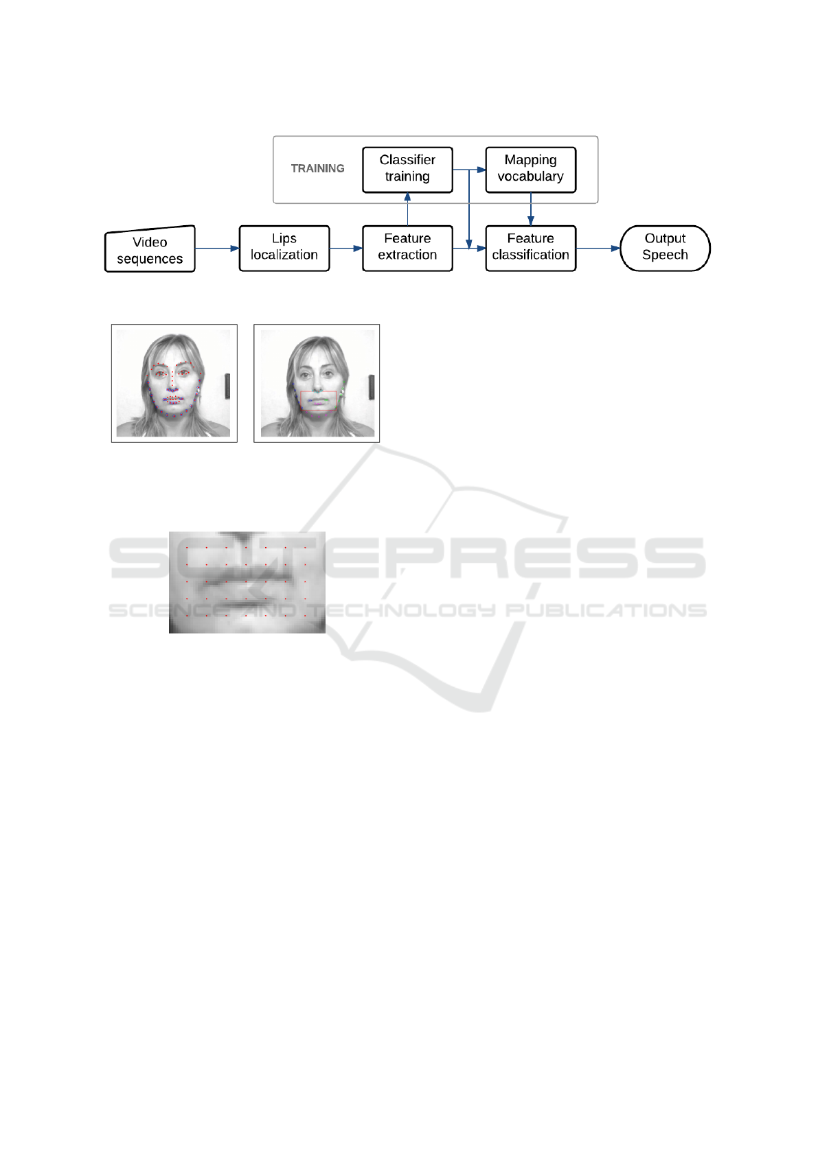
Figure 1: General process of a VASR system.
(a) (b)
Figure 2: (a) IOF-ASM detection, the marks in blue are
used to fix the bounding box; (b) ROI detection, each color
fix a lateral of the bounding box.
Figure 3: Keypoints distribution.
2.2.1 Lips Localization
The location of the face is obtained using invariant op-
timal features ASM (IOF-ASM) (Sukno et al., 2007)
that provides an accurate segmentation of the face in
frontal views. The face is tracked at every frame and
detected landmarks are used to fix a bounding box
around the lips (ROI) (Figure 2). At this stage the
ROI can have a different size in each frame. Thus,
ROIs are normalized to a fixed size of 48 × 64 pixels
to achieve a uniform representation.
2.2.2 Feature Extraction
After the ROI is detected a feature extraction stage
is performed. Nowadays, there is no universal fea-
ture for visual speech representation in contrast to
the Mel-frequency cepstral coefficients (MFCC) for
acoustic speech. We look for an informative fea-
ture invariant to common video issues, such as noise
or illumination changes. We analyze three different
appearance-based techniques:
• SIFT: SIFT was selected as high level descrip-
tor to extract the features in both the spatial and
temporal domains because it is highly distinctive
and invariant to image scaling and rotation, and
partially invariant to illumination changes and 3D
camera viewpoint (Lowe, 2004). In the spatial do-
main, the SIFT descriptor was applied directly to
the ROI, while in the temporal domain it was ap-
plied to the centred gradient. SIFT keypoints are
distributed uniformly around the ROI (Figure 3).
The distance between keypoints was fixed to half
of the neighbourhood covered by the descriptor
to gain robustness (by overlapping). As the di-
mension of the final descriptor for both spatial
and temporal domains is very high, PCA was ap-
plied to reduce the dimensionality of the features.
Only statistically significant components (deter-
mined by means of Parallel Analysis (Franklin
et al., 1995)) were retained.
• DCT: The 2D DCT is one of the most popular
techniques for feature extraction in visual speech
(Zhou et al., 2014b), (Lan et al., 2009). Its abil-
ity to compress the relevant information in a few
coefficients results in a descriptor with small di-
mensionality. The 2D DCT was applied directly
to the ROI. To fix the number of coefficients, the
image error between the original ROI and the re-
constructed was used. Based on preliminary ex-
periments, we found that 121 coefficients (corre-
sponding to 1% reconstruction error) for both the
spatial and temporal domains produced satisfac-
tory performance.
• PCA: Another popular technique is PCA, also
known as eigenlips (Zhou et al., 2014b), (Lan
et al., 2009), (Cappelletta and Harte, 2011). PCA,
as 2D DCT is applied directly to the ROI. To de-
cide the optimal number of dimensions the system
was trained and tested taking different percent-
ages of the total variance. Lower number of com-
Automatic Viseme Vocabulary Construction to Enhance Continuous Lip-reading
55
ponents would lead to a low quality reconstruc-
tion, but an excessive number of components will
be more affected by noise. In the end 90% of the
variance was found to be a good compromise and
was used in both spatial and temporal descriptors.
The early fusion of DCT-SIFT and PCA-SIFT has
been also explored to obtain a more robust descriptor
(see results in Section 3.3).
2.2.3 Feature Classification and Interpretation
The final goal of this block is to convert the extracted
features into phonemes or, if that is not possible, at
least into visemes. To this end we need: 1) classifiers
that will map features to (a first estimate of) visemes;
2) a mapping between phonemes and visemes; 3) a
model that imposes temporal coherency to the esti-
mated sequences.
1. Classifiers: classification of visemes is a chal-
lenging task, as it has to deal with issues such as
class imbalance and label noise. Several methods
have been proposed to deal with these problems,
the most common solutions being Bagging and
Boosting algorithms (Khoshgoftaar et al., 2011),
(Verbaeten and Van Assche, 2003), (Fr
´
enay and
Verleysen, 2014), (Nettleton et al., 2010). From
these, Bagging has been reported to perform bet-
ter in the presence of training noise and thus it was
selected for our experiments. Multiple LDA was
evaluated using cross validation. To add robust-
ness to the system, we trained classifiers to pro-
duce not just a class label but to estimate also a
class probability for each input sample.
For each bagging split, we train a multi-class LDA
classifier and use the Mahalanobis distance d to
obtain a normalized projection of the data into
each class c:
d
c
(x) =
q
(x − ¯x
c
)
T
· Σ
−1
c
· (x − ¯x
c
) (1)
Then, for each class, we compute two cumulative
distributions based on these projections: one for
in-class samples Φ(
d
c
(x)−µ
c
σ
c
), x ∈ c and another
one for out-of-class samples Φ(
d
c
(x)−µ
e
c
σ
e
c
), x ∈
e
c,
which we assume Gaussian with means µ
c
, µ
e
c
and
variances σ
c
, σ
e
c
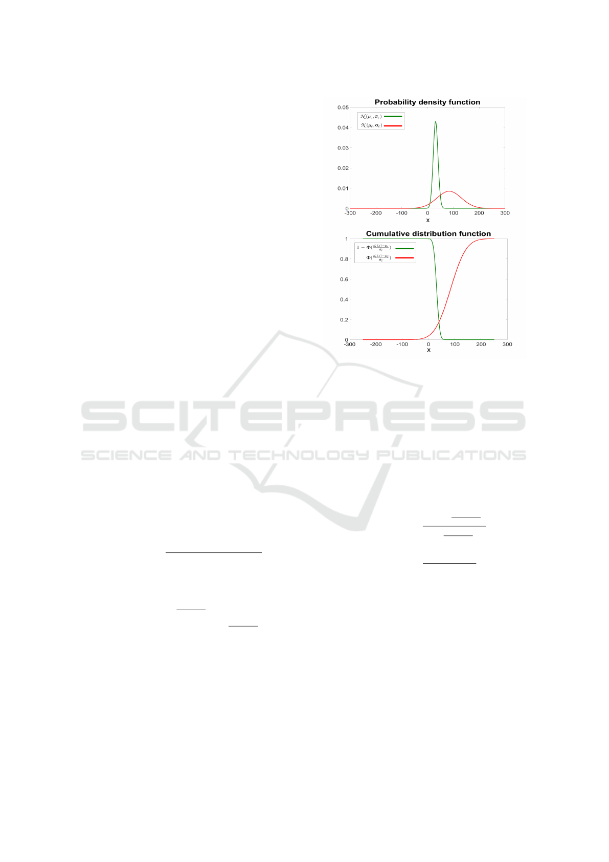
, respectively. An indicative ex-
ample is provided in Figure 4. Notice that these
means and variances correspond to the projections
in (1) and are different from ¯x
c
and Σ
c
.
We compute a class-likelihood as the ratio be-
tween the in-class and the out-of-class distribu-
tions, as in (2) and normalize the results so that the
summation over all classes is 1, as in (3). When
Figure 4: (Top) Probability density functions for in-class
(green) and out-of-class (red) samples; (Bottom) Cumula-
tive distributions corresponding to (Top). Notice than for
in-class samples we use the complement of the cumulative
distribution, since lower values should have higher proba-
bilities.
classifying a new sample, we use the cumulative
distributions to estimate the probability that the
unknown sample belongs to each of the viseme
classes (3). We assign the class with the highest
normalized likelihood L
c
.
F(c | x) =
1 − Φ(
d
c
(x)−µ
c
σ
c
)
Φ(
d
c
(x)−µ
e
c
σ
e
c
)
(2)
L
c
(x) =
F(c | x)
∑
C
c=1
F(c | x)
(3)
Once the classifiers are trained we could the-
oretically try to classify features directly into
phonemes, but as explained in Section 1, there are
phonemes that share the same visual appearance
and are therefore unlikely to be distinguishable
by a visual-only system. Thus, such phonemes
should be grouped into the same class (visemes).
In the next subsection we will present a map-
ping from phonemes to visemes based on group-
ing phonemes that are visually similar.
2. Phoneme to Viseme Mapping: to construct our
viseme to phoneme mapping we analyse the con-
fusion matrix resulting by comparing the ground
VISAPP 2017 - International Conference on Computer Vision Theory and Applications
56

truth labels of the training set with the automatic
classification obtained from the previous section.
We use an iterative process, starting with the same
number of visemes as phonemes, merging at each
step the visemes that show the highest ambigu-
ity. The method takes into account that vowels
cannot be grouped with consonants, because it
has been demonstrated that their aggregation pro-
duces worse results (Cappelletta and Harte, 2011),
(Bear et al., 2014).
The algorithm iterates until the desired vocabulary
length is achieved. However, there is no accepted
standard to fix this value beforehand. Indeed,
several different viseme vocabularies have been
proposed in the literature typically with lengths
between 11 and 15 visemes. Hence, in Section
3.3 we will analyse the effect of the vocabulary
size on recognition accuracy. Once the vocabu-
lary construction is concluded, all classifiers are
retrained based on the resulting viseme classes.
3. HMM and Viterbi Algorithm: to improve the
performance obtained after feature classification,
HMMs of one state per class are used to map: 1)
visemes to visemes; 2) visemes to phonemes.
An HMM λ = (A, B, π) is formed by N states
and M observations. Matrix A represents the
state transition probabilities, matrix B the emis-
sion probabilities, and vector π the initial state
probabilities. Given a sequence of observation O
and the model λ our aim is to find the maximum
probability state path Q = q
1
, q
2
, ..., q
t−1
. This can
be done recursively using Viterbi algorithm (Ra-
biner, 1989), (Petrushin, 2000). Let δ
i
(t) be the
probability of the most probable state path ending
in state i at time t (4). Then δ
j
(t) can be com-
puted recursively using (5) with initialization (6)
and termination (7).
δ
i
(t) = max
q
1
,...,q
t−1
P(q
1
...q
t−1
= i, O
1
, ..., O
t
|λ) (4)
δ
j
(t) = max
1≤i≤N
[δ
i
(t − 1) · a
i, j
] · b
j
(O
t
) (5)
δ
i
(1) = π
i
· b
i
(O
1
), 1 ≤ i ≤ N (6)
P = max
1≤i≤N
[δ
i
(T )] (7)
A shortage of the above is that it only considers a
single observation for each instant t. In our case
observations are the output from classifiers and
contain uncertainty. We have found that it is use-
ful to consider multiple possible observations for
each time step. We do this by adding to the Viterbi
algorithm the likelihoods obtained by the classi-
fiers for all classes (e.g. from equation (3)). As
a result, (5) is modified into (8), where the max-
imization is done across both the N states (as in
(5)) and also the M possible observations, each
weighted with its likelihood estimated by the clas-
sifiers.
δ
j
(t) = max
1≤O
t
≤M
max
1≤i≤N
[δ
i
(t − 1) · a
i, j
] ·
ˆ
b
j
(O
t
) (8)
ˆ
b
j
(O
t
) = b
j
(O
t
) · L(O
t
) (9)
where the short-form L(O
t
) refers to the likeli-
hood L
O
t
(x) as defined in (3). The Viterbi algo-
rithm modified as indicated in (8) is used to ob-
tain the final phoneme sequence providing at the
same time temporal consistency and tolerance to
classification uncertainties. Once this has been
achieved, visemes are mapped into phonemes us-
ing the traditional Viterbi algorithm (5).
3 EXPERIMENTS
3.1 Database
Ortega et al. (Ortega et al., 2004) introduced
AV@CAR as a free multichannel multi-modal
database for automatic audio-visual speech recogni-
tion in Spanish language, including both studio and
in-car recordings. The Audio-Visual-Lab data set of
AV@CAR contains sequences of 20 people recorded
under controlled conditions while repeating prede-
fined phrases or sentences. There are 197 sequences
for each person, recorded in AVI format. The video
data has a spatial resolution of 768x576 pixels, 24-
bit pixel depth and 25 fps and is compressed at an
approximate rate of 50:1. The sequences are divided
into 9 sessions and were captured in a frontal view
under different illumination conditions and speech
tasks. Session 2 is composed by 25 videos/user with
phonetically-balanced phrases. We have used session
2 splitting the dataset in 380 sentences (19 users ×
20 sentences/user) for training and 95 sentences (19
users × 5 sentences/user) to test the system. In Table
1 it is shown the sentences of the first speaker.
3.2 Phonetic Vocabulary
SAMPA is a phonetic alphabet developed in 1989
by an international group of phoneticians, and was
applied to European languages as Dutch, English,
French, Italian, Spanish, etc. We based our phonetic
vocabulary in SAMPA because it is the most used
standard in phonetic transcription (Wells et al., 1997),
Automatic Viseme Vocabulary Construction to Enhance Continuous Lip-reading
57
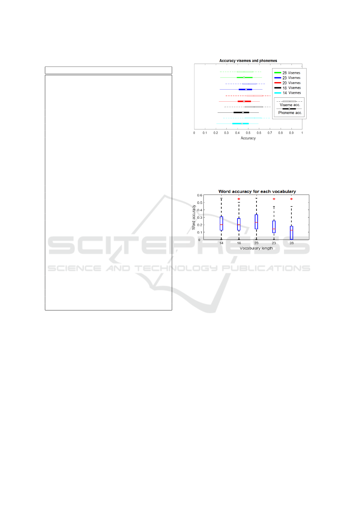
Table 1: Sentences for speaker 1.
Speaker 1
Francia, Suiza y Hungr
´
ıa ya hicieron causa
com
´
un.
Despu
´
es ya se hizo muy amiga nuestra.
Los yernos de Ismael no engordar
´
an los pollos con
hierba.
Despu
´
es de la mili ya me vine a Catalu
˜
na.
Bajamos un d
´
ıa al mercadillo de Palma.
Existe un viento del norte que es un viento fr
´
ıo.
Me he tomado un caf
´
e con leche en un bar.
Yo he visto a gente expulsarla del colegio por fu-
mar.
Guadalajara no est
´
a colgada de las rocas.
Pas
´
e un a
˜
no dando clase aqu
´
ı, en Bellaterra.
Pero t
´
u ahora elijes ya previamente.
Les dijeron que eligieran una casa all
´
a, en las mis-
mas condiciones.
Cuando me gir
´
e ya no ten
´
ıa la cartera.
Tendr
´
a unas siete u ocho islas alrededor.
Haciendo el primer campamento y el segundo
campamento.
Unas indemnizaciones no les iban del todo mal.
Rezando porque ten
´
ıa un miedo impresionante.
Es un apellido muy abundante en la zona de Pam-
plona.
No jug
´
abamos a b
´
asket, s
´
olo los mir
´
abamos a el-
los.
Aunque naturalmente hay un partido comunista.
Dio la casualidad que a la una y media estaban
all
´
ı.
Se alegraron mucho de vernos y ya nos quedamos
a cenar.
Ya empezamos a llorar bastante en el apartamento.
En una ladera del monte se ubica la iglesia.
Entonces lo
´
unico que hac
´
ıamos era ir a cenar.
(Llisterri and Mari
˜
no, 1993). For the Spanish lan-
guage, the vocabulary is composed by the following
29 phonemes: /p/, /b/, /t/, /d/, /k/, /g/, /tS/, /jj/, /f/,
/B/, /T/, /D/, /s/, /x/, /G/, /m/, /n/, /J/, /l/, /L/, /r/, /rr/,
/j/, /w/, /a/, /e/, /i/, /o/, /u/. The phonemes /jj/ and
/G/ were removed from our experiments because our
database did not contain enough samples to consider
them.
3.3 Results
In this section we show the results of our experi-
ments. In particular, we show the comparison of the
performances between the different vocabularies, the
different features, and the improvement obtained by
adding the observation probabilities into the Viterbi
algorithm.
Figure 5: Boxplots of system performance in terms of
phoneme and viseme accuracy for different vocabularies.
We analyze the one-to-one mapping phoneme to viseme,
and the one-to-many phoneme to viseme mappings with 23,
20, 16 and 14 visemes. The phoneme accuracy is always
computed from the 28 phonemes.
Figure 6: Comparison of system performance in word
recognition rate for the different vocabularies.
3.3.1 Experimental Setup
We constructed an automatic system that uses local
appearance features based on early fusion of DCT
and SIFT descriptors (this combination produced the
best results in our tests, see below) to extract the main
characteristics of the mouth region in both spatial and
temporal domains. The classification of the extracted
features into phonemes is done in two steps. Firstly,
100 LDA classifiers are trained using bagging se-
quences to be robust under label noise. Then, the clas-
sifier outputs are used to compute the global normal-
ized likelihood, as the summation over the normalized
likelihood computed by each classifier divided by the
number of classifiers (as explained in Section 2). Sec-
ondly, at the final step, one-state-per-class HMMs are
used to model the dynamic relations of the estimated
visemes and produce the final phoneme sequences.
3.3.2 Comparison of Different Vocabularies
As we explained before one of the main challenges
of VASR systems is the definition of the phoneme-to-
viseme mapping. While our system aims to estimate
VISAPP 2017 - International Conference on Computer Vision Theory and Applications
58
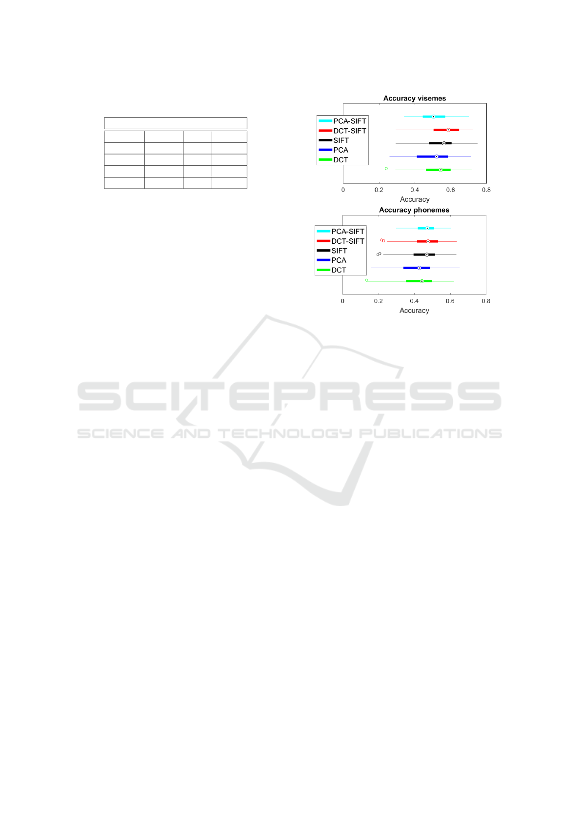
Table 2: Optimal vocabulary obtained, composed of 20
visemes.
Viseme vocabulary
Silence T l rr
D ll d s, tS, t
k x j r
g m, p, b f n
B J a,e,i o,u,w
phoneme sequences, we know that there is no one-to-
one mapping between phonemes and visemes. Hence,
we try to find the one-to-many mapping that will al-
low us to maximize the recognition of phonemes in
the spoken message.
To evaluate the influence of the different map-
pings, we have analysed the performance of the sys-
tem in terms of viseme- , phoneme-, and word recog-
nition rates using viseme vocabularies of different
lengths. Our first observation, from Figure 5, is
that the viseme accuracy tends to grow as we re-
duce the vocabulary length. This is explained by
two factors: 1) the reduction in number of classes,
which makes the classification problem a simpler one
to solve; 2) the fact that visually indistinguishable
units are combined into one. The latter helps ex-
plain the behaviour of the other metric in the fig-
ure: phoneme accuracy. As we reduce the vocab-
ulary length, phoneme accuracy firstly increases be-
cause we eliminate some of the ambiguities by merg-
ing visually similar units. But if we continue to re-
duce the vocabulary, too many phonemes (even unre-
lated) are mixed together and their accuracy decreases
because, even if these visemas are better recognized,
their mapping into phonemes is more uncertain. Thus,
the optimal performance is obtained for intermediate
vocabulary lengths, because there is an optimum com-
promise between the visemes and the phonemes that
can be recognized.
The same effect can also be seen in Figure 6 in
terms of word recognition rates. We can observe how
the one-to-one phoneme to viseme mapping (using
the 28 phonemes classes) obtained the lowest word
recognition rates and how the highest word recogni-
tion rates were obtained for the intermediate vocabu-
lary lengths, supporting the view that the one-to-many
mapping from phonemes to visemes is necessary to
optimize the performance of visual speech systems.
In the experiments presented in this paper, a vocabu-
lary of 20 visemes (summarized in Table 2) produced
the best performance.
Figure 7: Comparison of features performance.
3.3.3 Feature Comparison
To analyse the performance of the different features
we have fixed the viseme vocabulary as shown in Ta-
ble 2 and performed a 4-fold cross-validation on the
training set. We used 100 LDA classifiers per fold,
generated by means of a bagging strategy. Figure 7
displays the results. Visualizing the features indepen-
dently, DCT and SIFT give the best performances.
The fusion of both features produced an accuracy of
0.58 for visemes, 0.47 for phonemes.
3.3.4 Improvement by Adding Classification
Likelihoods
Figure 8 shows how the accuracy varies when con-
sidering the classifier likelihoods in the Viterbi algo-
rithm. The horizontal axis indicates the number of
classes that are considered (the rank), in decreasing
order of likelihood. The performance of the algorithm
without likelihoods (5) is also provided as a baseline
(rank 0). We see that the improvement obtained by
the inclusion of class likelihoods is up to 20%.
Finally, it is interesting to analyse how the sys-
tem performs for each of the resulting phonemes. Fig-
ure 9 (a) shows the frequency of appearance of each
phoneme. In Figure 9 (b) we show the number of
phonemes that are wrongly detected. It can be seen
that the input data is highly unbalanced, biasing the
system toward the phonemes that appear more often.
For example, the silence appears 4 times more than
the vowels a,e,i and there are some phonemes with
Automatic Viseme Vocabulary Construction to Enhance Continuous Lip-reading
59
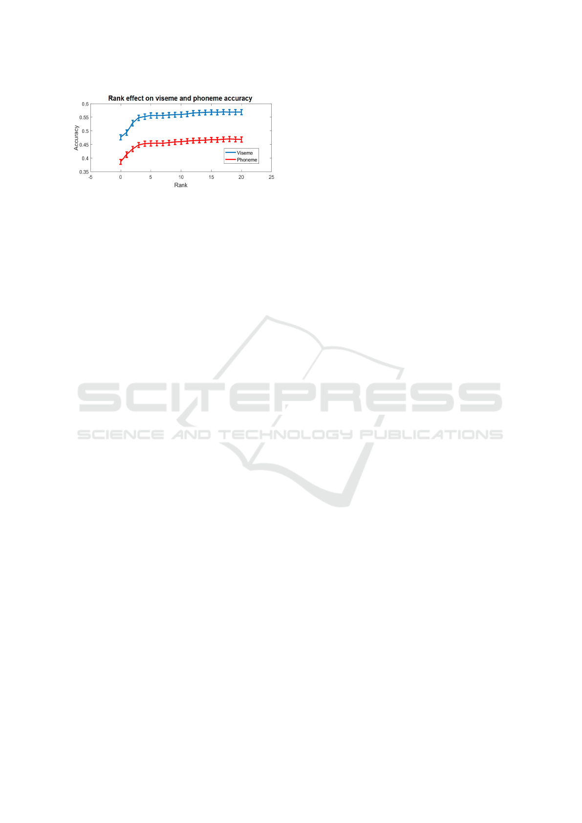
Figure 8: Accuracy for different ranks in the Viterbi algo-
rithm.
very few samples, such as rr, f or b. This has also
an impact in terms of precision and recall, as can be
observed in Figure 9 (c). In the precision and re-
call figure we can observe the effects of the many-
to-one viseme to phoneme mapping. For example,
there are phonemes with low precision and recall be-
cause have been confused with one of the phonemes
of their viseme group (e.g: vowel i have been con-
fused with a and e). Considering the three plots at
once, there is a big impact of the silence on the overall
performance of the system. In particular, the recogni-
tion of silences shows a very high precision but its
recall is only about 70%. By inspecting our data, we
found that this is easily explained by the fact that, nor-
mally, people start moving their lips before speaking,
in preparation for the upcoming utterance. Combina-
tion with audio would easily resolve this issue.
4 CONCLUSIONS
We investigate the automatic construction of op-
timal viseme vocabularies by iteratively combin-
ing phonemes with similar visual appearance into
visemes. We perform tests on the Spanish database
AV@CAR using a VASR system based on the com-
bination of DCT and SIFT descriptors in spatial and
temporal domains and HMMs to model both viseme
and phoneme dynamics. Using 19 different speakers
we reach a 58% of recognition accuracy in terms of
viseme units, 47% in terms of phoneme units and 23%
in terms of words units, which is remarkable for a
multi-speaker dataset of continuous speech as the one
used in our experiments. Comparing the performance
obtained by our viseme vocabulary with the perfor-
mance of other vocabularies, such as those analysed
by Cappelleta et al. in (Cappelletta and Harte, 2011),
we observe that the 4 vocabularies they propose have
lengths of 11, 12, 14 and 15 visemes and their maxi-
mum accuracy is between 41% and 60% (in terms of
viseme recognition).
Interestingly, while our results support the advan-
tage of combining multiple phonemes into visemes to
improve performance, the number of visemes that we
obtain are comparatively high with respect to previous
efforts. In our case, the optimal vocabulary length for
Spanish reduced from 28 phonemes to 20 visemes (in-
cluding Silence), i.e. a reduction rate of about 3 : 2. In
contrast, previous efforts reported for English started
from 40 to 50 phonemes and merged them into just
11 to 15 visemes (Cappelletta and Harte, 2011), with
reduction rates from 3 : 1 to 5 : 1. It is not clear,
however, if the higher compression of the vocabular-
ies obeys to a difference inherent to language or to
other technical aspects, such as the ways of defining
the phoneme to viseme mapping.
Indeed, language differences make it difficult to
make a fair comparison of our results with respect to
previous work. Firstly, it could be argued that our
viseme accuracy is comparable to values reported by
Cappelletta et al. (Cappelletta and Harte, 2011); how-
ever they used at most 15 visemes while we use 20
visemes and, as shown in Figure 5, when the num-
ber of visemes decreases, viseme recognition accu-
racy increases but phoneme accuracy might be re-
duced hence making more difficult to recover the spo-
ken message. Unfortunately, Cappelletta et al. (Cap-
pelletta and Harte, 2011) did not report their phoneme
recognition rates.
Another option for comparison is word-
recognition rates, which are frequently reported
in automatic speech recognition systems. However,
in many cases recognition rates are reported only for
audio-visual systems without indicating visual-only
performance (Hazen et al., 2004), (Cooke et al.,
2006). Within systems reporting visual-only perfor-
mance, comparison is also difficult given that they
are often centered on tasks such as digit or sentence
recognition (Seymour et al., 2008), (Sui et al., 2015),
(Zhao et al., 2009), (Saenko et al., 2005), which
are considerably simpler than the recognition of
continuous speech, as addressed here. Focusing on
continuous systems for visual speech, Cappelleta et
al. (Cappelletta and Harte, 2011) did not report word
recognition rates and Thangthai et al. (Thangthai
et al., 2015) reported tests just on a single user.
Finally, Potamianos et al. (Potamianos et al., 2003)
implemented a system comparable to ours based on
appearance features and tested it using the multi-
speaker IBM ViaVoice database, achieving 17.49%
of word recognition rate in continuous speech, which
is not far from the 23% of word recognition rate
achieved by our system.
VISAPP 2017 - International Conference on Computer Vision Theory and Applications
60
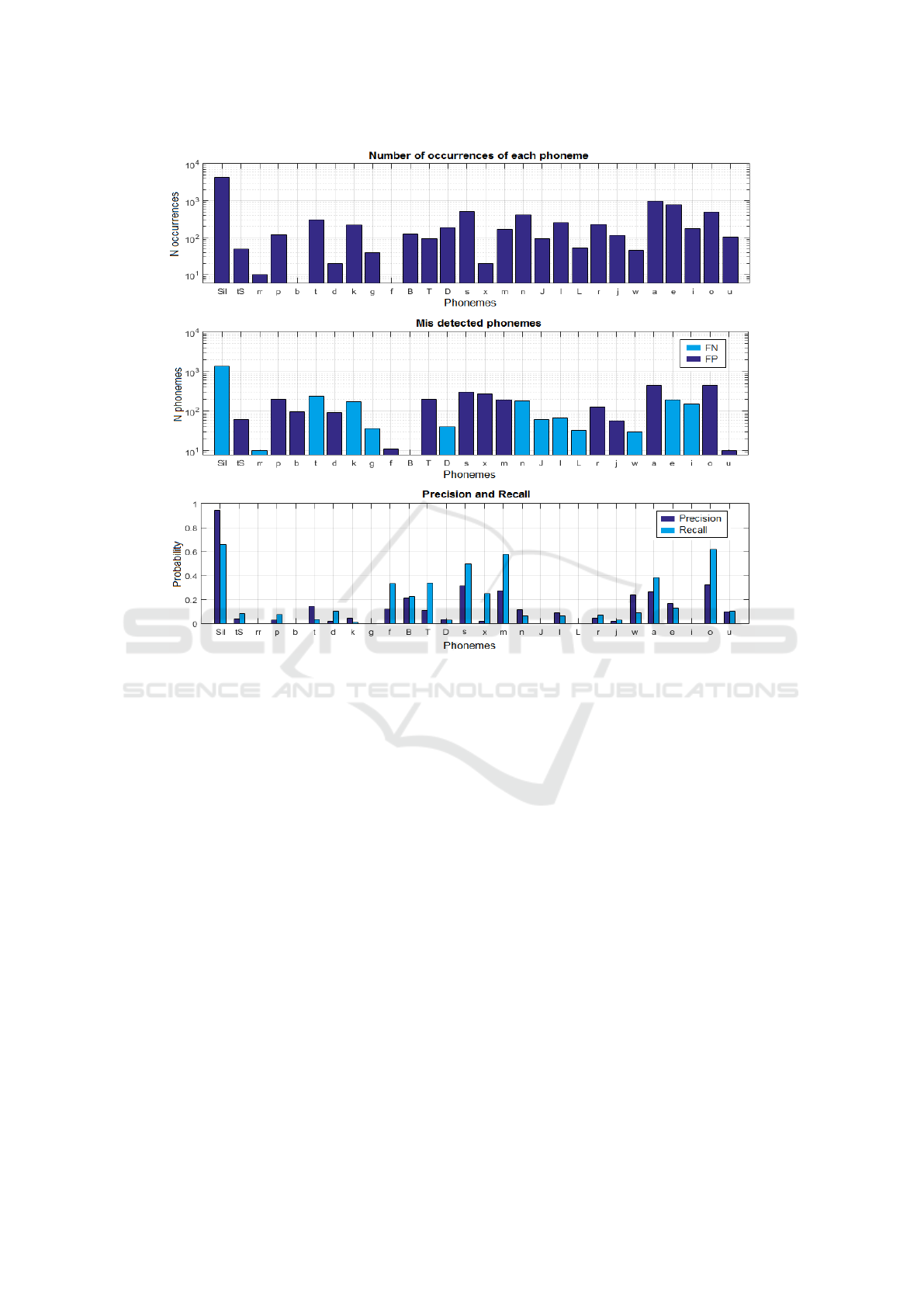
Figure 9: (a) Number of occurrences of each viseme; (b) Visemes wrongly detected (actual - detected), light blue (false
negatives) and dark blue (false positives); (c) Precision and Recall of visemes.
ACKNOWLEDGEMENTS
This work is partly supported by the Spanish Ministry
of Economy and Competitiveness under the Ramon y
Cajal fellowships and the Maria de Maeztu Units of
Excellence Programme (MDM-2015-0502), and the
Kristina project funded by the European Union Hori-
zon 2020 research and innovation programme under
grant agreement No 645012.
REFERENCES
Antonakos, E., Roussos, A., and Zafeiriou, S. (2015). A sur-
vey on mouth modeling and analysis for sign language
recognition. In Automatic Face and Gesture Recogni-
tion (FG), 2015 11th IEEE International Conference
and Workshops on, volume 1, pages 1–7. IEEE.
Bear, H. L., Harvey, R. W., Theobald, B.-J., and Lan, Y.
(2014). Which phoneme-to-viseme maps best im-
prove visual-only computer lip-reading? In Interna-
tional Symposium on Visual Computing, pages 230–
239. Springer.
Bozkurt, E., Erdem, C. E., Erzin, E., Erdem, T., and Ozkan,
M. (2007). Comparison of phoneme and viseme based
acoustic units for speech driven realistic lip animation.
Proc. of Signal Proc. and Communications Applica-
tions, pages 1–4.
Buchan, J. N., Par
´
e, M., and Munhall, K. G. (2007). Spatial
statistics of gaze fixations during dynamic face pro-
cessing. Social Neuroscience, 2(1):1–13.
Cappelletta, L. and Harte, N. (2011). Viseme definitions
comparison for visual-only speech recognition. In
Signal Processing Conference, 2011 19th European,
pages 2109–2113. IEEE.
Chit¸u, A. and Rothkrantz, L. J. (2012). Automatic vi-
sual speech recognition. Speech enhancement, Mod-
eling and Recognition–Algorithms and Applications,
page 95.
Cooke, M., Barker, J., Cunningham, S., and Shao, X.
(2006). An audio-visual corpus for speech perception
and automatic speech recognition. The Journal of the
Acoustical Society of America, 120(5):2421–2424.
Dupont, S. and Luettin, J. (2000). Audio-visual speech
modeling for continuous speech recognition. IEEE
transactions on multimedia, 2(3):141–151.
Erber, N. P. (1975). Auditory-visual perception of speech.
Automatic Viseme Vocabulary Construction to Enhance Continuous Lip-reading
61

Journal of Speech and Hearing Disorders, 40(4):481–
492.
Ezzat, T. and Poggio, T. (1998). Miketalk: A talking fa-
cial display based on morphing visemes. In Computer
Animation 98. Proceedings, pages 96–102. IEEE.
Fisher, C. G. (1968). Confusions among visually perceived
consonants. Journal of Speech, Language, and Hear-
ing Research, 11(4):796–804.
Franklin, S. B., Gibson, D. J., Robertson, P. A., Pohlmann,
J. T., and Fralish, J. S. (1995). Parallel analysis: a
method for determining significant principal compo-
nents. Journal of Vegetation Science, 6(1):99–106.
Fr
´
enay, B. and Verleysen, M. (2014). Classification in the
presence of label noise: a survey. IEEE transactions
on neural networks and learning systems, 25(5):845–
869.
Goldschen, A. J., Garcia, O. N., and Petajan, E. (1994).
Continuous optical automatic speech recognition by
lipreading. In Signals, Systems and Computers, 1994.
1994 Conference Record of the Twenty-Eighth Asilo-
mar Conference on, volume 1, pages 572–577. IEEE.
Hazen, T. J., Saenko, K., La, C.-H., and Glass, J. R.
(2004). A segment-based audio-visual speech recog-
nizer: Data collection, development, and initial exper-
iments. In Proceedings of the 6th international confer-
ence on Multimodal interfaces, pages 235–242. ACM.
Hilder, S., Harvey, R., and Theobald, B.-J. (2009). Com-
parison of human and machine-based lip-reading. In
AVSP, pages 86–89.
Jeffers, J. and Barley, M. (1980). Speechreading (lipread-
ing). Charles C. Thomas Publisher.
Khoshgoftaar, T. M., Van Hulse, J., and Napolitano, A.
(2011). Comparing boosting and bagging techniques
with noisy and imbalanced data. IEEE Transactions
on Systems, Man, and Cybernetics-Part A: Systems
and Humans, 41(3):552–568.
Lan, Y., Harvey, R., Theobald, B., Ong, E.-J., and Bow-
den, R. (2009). Comparing visual features for lipread-
ing. In International Conference on Auditory-Visual
Speech Processing 2009, pages 102–106.
Llisterri, J. and Mari
˜
no, J. B. (1993). Spanish adaptation of
sampa and automatic phonetic transcription. Reporte
t
´
ecnico del ESPRIT PROJECT, 6819.
Lowe, D. G. (2004). Distinctive image features from scale-
invariant keypoints. International journal of computer
vision, 60(2):91–110.
Luettin, J., Thacker, N. A., and Beet, S. W. (1996). Visual
speech recognition using active shape models and hid-
den markov models. In Acoustics, Speech, and Signal
Processing, 1996. ICASSP-96. Conference Proceed-
ings., 1996 IEEE International Conference on, vol-
ume 2, pages 817–820. IEEE.
McGurk, H. and MacDonald, J. (1976). Hearing lips and
seeing voices. Nature, 264:746–748.
Moll, K. L. and Daniloff, R. G. (1971). Investigation of the
timing of velar movements during speech. The Jour-
nal of the Acoustical Society of America, 50(2B):678–
684.
Nefian, A. V., Liang, L., Pi, X., Xiaoxiang, L., Mao, C.,
and Murphy, K. (2002). A coupled hmm for audio-
visual speech recognition. In Acoustics, Speech, and
Signal Processing (ICASSP), 2002 IEEE International
Conference on, volume 2, pages II–2013. IEEE.
Neti, C., Potamianos, G., Luettin, J., Matthews, I., Glotin,
H., Vergyri, D., Sison, J., and Mashari, A. (2000).
Audio visual speech recognition. Technical report,
IDIAP.
Nettleton, D. F., Orriols-Puig, A., and Fornells, A. (2010).
A study of the effect of different types of noise on the
precision of supervised learning techniques. Artificial
intelligence review, 33(4):275–306.
Ortega, A., Sukno, F., Lleida, E., Frangi, A. F., Miguel, A.,
Buera, L., and Zacur, E. (2004). Av@ car: A spanish
multichannel multimodal corpus for in-vehicle auto-
matic audio-visual speech recognition. In LREC.
Ortiz, I. d. l. R. R. (2008). Lipreading in the prelingually
deaf: what makes a skilled speechreader? The Spanish
journal of psychology, 11(02):488–502.
Pei, Y., Kim, T.-K., and Zha, H. (2013). Unsupervised
random forest manifold alignment for lipreading. In
Proceedings of the IEEE International Conference on
Computer Vision, pages 129–136.
Petrushin, V. A. (2000). Hidden markov models: Funda-
mentals and applications. In Online Symposium for
Electronics Engineer.
Potamianos, G., Neti, C., Gravier, G., Garg, A., and Se-
nior, A. W. (2003). Recent advances in the automatic
recognition of audiovisual speech. Proceedings of the
IEEE, 91(9):1306–1326.
Rabiner, L. R. (1989). A tutorial on hidden markov models
and selected applications in speech recognition. Pro-
ceedings of the IEEE, 77(2):257–286.
Ronquest, R. E., Levi, S. V., and Pisoni, D. B. (2010). Lan-
guage identification from visual-only speech signals.
Attention, Perception, & Psychophysics, 72(6):1601–
1613.
Saenko, K., Livescu, K., Siracusa, M., Wilson, K., Glass,
J., and Darrell, T. (2005). Visual speech recognition
with loosely synchronized feature streams. In Tenth
IEEE International Conference on Computer Vision
(ICCV’05) Volume 1, volume 2, pages 1424–1431.
Sahu, V. and Sharma, M. (2013). Result based analysis
of various lip tracking systems. In Green High Per-
formance Computing (ICGHPC), 2013 IEEE Interna-
tional Conference on, pages 1–7. IEEE.
Seymour, R., Stewart, D., and Ming, J. (2008). Comparison
of image transform-based features for visual speech
recognition in clean and corrupted videos. Journal on
Image and Video Processing, 2008:14.
Sui, C., Bennamoun, M., and Togneri, R. (2015). Listen-
ing with your eyes: Towards a practical visual speech
recognition system using deep boltzmann machines.
In Proceedings of the IEEE International Conference
on Computer Vision, pages 154–162.
Sukno, F. M., Ordas, S., Butakoff, C., Cruz, S., and Frangi,
A. F. (2007). Active shape models with invariant op-
timal features: application to facial analysis. IEEE
Transactions on Pattern Analysis and Machine Intel-
ligence, 29(7):1105–1117.
VISAPP 2017 - International Conference on Computer Vision Theory and Applications
62

Sumby, W. H. and Pollack, I. (1954). Visual contribution
to speech intelligibility in noise. The journal of the
acoustical society of america, 26(2):212–215.
Thangthai, K., Harvey, R., Cox, S., and Theobald, B.-J.
(2015). Improving lip-reading performance for robust
audiovisual speech recognition using dnns. In Proc.
FAAVSP, 1St Joint Conference on Facial Analysis, An-
imation and Audio–Visual Speech Processing.
Verbaeten, S. and Van Assche, A. (2003). Ensemble meth-
ods for noise elimination in classification problems.
In International Workshop on Multiple Classifier Sys-
tems, pages 317–325. Springer.
Wells, J. C. et al. (1997). Sampa computer readable pho-
netic alphabet. Handbook of standards and resources
for spoken language systems, 4.
Yau, W. C., Kumar, D. K., and Weghorn, H. (2007). Visual
speech recognition using motion features and hidden
markov models. In International Conference on Com-
puter Analysis of Images and Patterns, pages 832–
839. Springer.
Zhao, G., Barnard, M., and Pietikainen, M. (2009). Lipread-
ing with local spatiotemporal descriptors. IEEE
Transactions on Multimedia, 11(7):1254–1265.
Zhou, Z., Hong, X., Zhao, G., and Pietik
¨
ainen, M. (2014a).
A compact representation of visual speech data using
latent variables. IEEE transactions on pattern analy-
sis and machine intelligence, 36(1):1–1.
Zhou, Z., Zhao, G., Hong, X., and Pietik
¨
ainen, M. (2014b).
A review of recent advances in visual speech decod-
ing. Image and vision computing, 32(9):590–605.
Automatic Viseme Vocabulary Construction to Enhance Continuous Lip-reading
63
