
Near Real-time Object Detection in RGBD Data
Ronny H
¨
ansch, Stefan Kaiser and Olaf Helwich
Computer Vision & Remote Sensing, Technische Universit
¨
at Berlin, Berlin, Germany
Keywords:
Object Detection, Random Forests, RGBD-data.
Abstract:
Most methods of object detection with RGBD cameras set hard constraints on their operational area. They
only work with specific objects, in specific environments, or rely on time consuming computations. In the
context of home robotics, such hard constraints cannot be made. Specifically, an autonomous home robot
shall be equipped with an object detection pipeline that runs in near real-time and produces reliable results
without restricting object type and environment. For this purpose, a baseline framework that works on RGB
data only is extended by suitable depth features that are selected on the basis of a comparative evaluation. The
additional depth data is further exploited to reduce the computational cost of the detection algorithm. A final
evaluation of the enhanced framework shows significant improvements compared to its original version and
state-of-the-art methods in terms of both, detection performance and real-time capability.
1 INTRODUCTION AND
RELATED WORK
Recent advances in robotics allow research to focus
on the potential integration of mobile manipulators
into home environments. One task of such robots
is to fetch and carry objects by utilising informa-
tion that are managed and stored by smart home sys-
tems.The task is subdivided into five steps: Search
object, estimate object pose, grip object, carry ob-
ject, and release-object. For a successful execution,
the robot needs to be equipped with a reliable object
detection algorithm that is able to cope with several
challenges including multiple object categories, only
weakly constrained object types,object poses with
six degrees of freedom, scenes cluttered by every-
day household objects, various backgrounds, chang-
ing object appearances due to different lighting con-
ditions, and a near real-time performance while main-
taining high detection accuracy.
Fulfilling all these requirements is a hard chal-
lenge, which is usually approached by equipping mo-
bile manipulators with multiple sensors, i.e. depth
and RGB cameras. While depth data is complemen-
tary to RGB images, their joint usage has its own chal-
lenges such as a higher computational load.
A sophisticated object detection toolkit for robot
manipulation tasks is proposed in (M
¨
orwald et al.,
2010). An edge-based tracker aligns a given 3D CAD
model of the object, such that its projection fits the
training object in the image. Distinctive SIFT feature
points are extracted and stored in a codebook along
with their three-dimensional coordinates on the model
surface. During the detection phase, SIFT points are
extracted from the scene and and matched against the
entries in the codebook. In (Tombari and Di Stefano,
2010) a 3D Hough voting scheme is used to local-
ize objects in point clouds. It is based on 3D fea-
ture points that have been extracted from the point
cloud of the object. For each feature point a local
reference frame and offset vector to the object’s cen-
ter are stored. For detection, feature points are ex-
tracted from the scene and matched against model
feature points which leads to a set of point-to-point
correspondences. The scene feature points vote into
a 3D Hough space by using the stored local reference
frame as well as the offset vector. Both methods re-
port state-of-the-art recognition and pose estimation
results. However, they lack several of the require-
ments for our work since not all object types can be
described well by feature points: While the perfor-
mance in (M
¨
orwald et al., 2010) drastically decreases
for objects at different scales or weakly textured sur-
faces, the used 3D detector in (Tombari and Di Ste-
fano, 2010) fails for simple shapes (such as boxes).
Template-based approaches utilize modalities
such as object shape and thus perform well for objects
without distinctive surface features. Early approaches
are based on matching each trained object template
with the image or its Fourier-transformation in a slid-
ing window approach (Vergnaud, 2011). A huge
HÃd’nsch R., Kaiser S. and Helwich O.
Near Real-time Object Detection in RGBD Data.
DOI: 10.5220/0006101401790186
In Proceedings of the 12th International Joint Conference on Computer Vision, Imaging and Computer Graphics Theory and Applications (VISIGRAPP 2017), pages 179-186
ISBN: 978-989-758-226-4
Copyright
c
2017 by SCITEPRESS – Science and Technology Publications, Lda. All rights reser ved
179

speedup is achieved in (Hinterstoisser et al., 2010)
by quantising image gradients from the templates.
LINEMOD (Hinterstoisser et al., 2011) extends this
work by adding depth features and is able detect an
impressive amount of objects simultaneously in near
real-time However, it produces many false positives in
cluttered scenes which requires time consuming post-
processing steps. The more recent works of (Hin-
terstoisser et al., 2013; Rios-Cabrera and Tuytelaars,
2013) additionally include color information. The
work in (Rusu et al., 2010) and its extension (Wang
et al., 2013) are operating on the point cloud level
(instead of intensity and depth image) and compute
viewpoint dependent feature histograms. During de-
tection, the learnt histograms are matched against his-
tograms of point cloud regions. The use case is re-
stricted to tabletop scenarios in which all objects re-
side on the dominant plane in the scene which allows
an easy foreground-background segmentation.
Recently, convolutional networks have been suc-
cessfully applied to RGBD tasks, such as learning
representations from depth images.The multiscale se-
mantic segmentation of (Farabet et al., 2013) is ex-
tended in (Couprie et al., 2013) to work directly on
RGBD images. The work in (Gupta et al., 2014) uses
a large convolutional network that was pre-trained on
RGB images to generate features for depth images
and obtains a substantial improvement of detection
accuracy. In (Bo et al., 2014) hierarchical match-
ing pursuit is used instead of deep nets to learn fea-
tures from images captured by RGBD cameras. These
works focus on detection accuracy and seldom make
statements about run time and computational costs.
The Implicit Shape Model (ISM) (Leibe et al.,
2006) applies a Hough voting scheme based on a
codebook of “visual words”, i.e. clustered image
patches, along with 2D offset vectors that cast prob-
abilistic votes for object centres. A 3D version of
ISM is proposed in (Knopp et al., 2010) where 3D
features and a 3D Hough space replace its 2D coun-
terparts. Both versions rely on feature point detec-
tors to reduce the search space leading to similar re-
strictions as discussed above. Hough Forests (Gall
et al., 2012) also learn to distinguish patches and cor-
responding offset vectors but do not use any feature
detector to find salient object locations. While a ran-
domized subset of object patches is sampled during
training, a sliding window is used during the detec-
tion stage. A Random Forest replaces patch cluster-
ing and codebook. The learning procedure aims to
distinguish patches of different classes (classification)
and to merge patches with similar offset vectors (re-
gression) simultaneously. The Hough Forest comes
with several desirable properties: 1) The Hough vot-
ing produces probabilistic object hypotheses. 2) The
distinctive training of objects against other objects
(and background) leads to potentially low false posi-
tive rates. 3) No object-type, -texture, -shape, scene or
background assumptions are made. 4) The framework
is independent of specific image features. 5) Perspec-
tive invariance is achieved by feeding training images
of different view points. Scale invariance is achieved
by resizing the query image. The downside of this ap-
proach is that detection time scales rather poorly with
image resolution, the maximum tree depth, as well as
the number of classes, scales, and trees. The work of
(Badami et al., 2013) uses a Hough Forest which is
trained jointly on image and depth features.However,
the individual contribution of the different features
is not analyzed, although it is noted that the usage
of depth features increases performance significantly
over using color information only. Furthermore, the
run time of the approach is not considered.
Our work focuses on leveraging the advantages of
Hough Forests for the object detection step of the full
pipeline while decreasing the computation time. To
reach reasonable classification results, the potential
of several depth-based features (Section 3) is investi-
gated by evaluating their individual classification ac-
curacies (Section 4). Based on these results, a final
set of features is proposed. Several methodological as
well as implementational adjustments reduce the time
complexity (Section 5) and enable near real-time per-
formance, while still achieving state-of-the-art detec-
tion accuracy (Section 6).
2 HOUGH FOREST
Hough Forests (Gall et al., 2012) are a variant of Ran-
dom Forests (Breiman, 2001) which is an ensemble
learning framework capable of classification and re-
gression. Similar to the Generalised Hough Trans-
form (Ballard, 1981), a Hough Forest accumulates
probabilistic object hypotheses in a voting space that
is parameterized by the object’s center (x, y), class c,
and scale s. Object candidates (c, x, y, s, p, b)
i
are ex-
tracted as maxima in this voting space, where p is
the candidate’s confidence. The candidate’s bound-
ing box b is estimated by backprojecting patches that
voted for this candidate. A post-processing step re-
moves detections whose bounding box overlaps an-
other detection with a significantly higher confidence
value.
Our work builds on the implementation of (Gall
et al., 2012) which is adapted as described in Sec-
tion 5 and extended by using a different set of features
(see Section 4).
VISAPP 2017 - International Conference on Computer Vision Theory and Applications
180

3 FEATURES
The following features are analyzed with respect to
classification performance and computational load in
Section 4:
1. Intensity-based Features. The implementation
of (Gall et al., 2012) uses minimal and maximal
values in a 5 × 5 pixel neighbourhood of the first
and second derivatives of the grayscale image and
the Histogram of Oriented Gradients (HOG) re-
sulting in a 32 dimensional feature vector.
2. Depth Value. As suggested in (Lai et al., 2011a)
the raw depth value d relative to the object size is
used, where the object size is replaced by scale s.
The scale-dependent depth value f
ds
= d · s mod-
els the direct proportionality between object dis-
tance and scale.
3. Depth Derivatives. The first and second order
derivatives of the (raw) depth value are computed
by the Sobel filter.
4. Depth HoG. While (Janoch et al., 2011) claims
that HoG on depth images falls behind its RGB
version, the Depth HoG outperforms the RGB
variant in (Lai et al., 2011a).
5. Histogram of Oriented Normal Vectors. The
Histogram of Oriented Normal Vectors (HONV,
(Tang et al., 2013)) extends the HoG by one
dimension and bins surface normals of a k-
neighbourhood into a two-dimensional histogram.
6. Principal Curvature. This feature describes the
local surface geometry in terms of minimal and
maximal curvature, corresponding to the eigen-
values of the covariance matrix of all points in a
k-neighbourhood projected onto the tangent plane
of the surface at a point (Arbeiter et al., 2012).
The vector indicating the direction of the maxi-
mum curvature (principal direction) contains fur-
ther surface information. To distinguish further
between curved surfaces, (Arbeiter et al., 2012)
suggests to use the ratio of minimum and maxi-
mum principal curvature.
7. (Fast) Point Feature Histograms. The Point
Feature Histogram (PFH) encodes shape proper-
ties by quantizing the geometrical relationship be-
tween pairs of points within the k-neighbourhood
of a query point (Rusu et al., 2009). While the
computational complexity of PFH is O(nk
2
) for a
point cloud with n points, its extension Fast Point
Feature Histogram (FPFH) reduces it to O(nk).
As for the RGB features, the minimum and maximum
in a 5× 5 neighbourhood is used for the scaled depth,
the depth derivatives, and the principal curvature.
4 FEATURE EVALUATION
The RGBD Object Dataset (Lai et al., 2011a) contains
about 300 objects in 51 categories recorded from vari-
ous perspectives. Each frame consists of an RGB and
a depth image, a bounding box, and a pixel-wise ob-
ject mask. The dataset provides indoor background
data and eight different annotated indoor scenes.
The scene table small 1 (Figure 3(a)) is used as
test set for the following comparisons due to its va-
riety of scene properties such as object size, surface
flatness and texture, object-camera distances, and per-
spectives. It contains four objects: A bowl, a cereal
box, a coffee mug, and a soda can. The training data
consists of 36 images of a full 360
◦
rotation for three
different pitch angles.The background data contains
215 images of ordinary office scenes, partly covering
the test set background but without the objects.
The evaluation results are reported as the area un-
der the precision/recall curves (AUC) over all frames
of the test scene. A detection is counted as true pos-
itive if the overlap of predicted and reference bound-
ing box is at least 50% of the joint area. The average
AUC is computed as mean over five training and test
runs.Multiple detections of the same object are con-
sidered as false positives.
The following standard parameters are used: 15
trees with a maximum depth of 25 levels, five scales
(0.33, 0.66, 1.0, 1.66, 2.33) with a query image res-
olution of 640 × 320, 250 patches of size 16 × 16
pixel are sampled from each training image. To get a
rich precision/recall evaluation, up to 250 detections
per class are allowed if they are above the detection
threshold of 0.1. All these parameters stay unchanged
during the following experiments and only the feature
space is modified by using the different depth features
(Section 3.2-7) additionally to the RGB features of
Section 3.1. The reported changes in performance are
always relative to the baseline of using only RGB.
1. RGB Features. The baseline detection perfor-
mance is an average AUC of 0.576. Figure 1(a)
shows that coffee mug and soda already perform
decent, while bowl and cereal box are far below
0.5. None of the objects reaches a perfect recall
and only coffee mug and soda can achieve a pre-
cision of 1.0 (coffee mug only at a very low re-
call). The non-monotonous trends of the bowl
and cereal box curves are caused by false detec-
tions with high confidence values. There are sev-
eral reasons for the bad performance of bowl and
cereal box. The bowl does not have any texture
which can be described by the intensity gradient
based feature vector. Only color and shape infor-
mation are useful here. The surface is reflective
Near Real-time Object Detection in RGBD Data
181

0.0 0.2 0.4 0.6 0.8 1.0
recall
0.0
0.2
0.4
0.6
0.8
1.0
precision
bowl_4: 0.354
cereal_box_1: 0.418
coffee_mug_1: 0.671
soda_can_3: 0.845
mean 0.576
(a) Baseline
0.0 0.2 0.4 0.6 0.8 1.0
recall
0.0
0.2
0.4
0.6
0.8
1.0
precision
bowl_4: 0.614
cereal_box_1: 0.881
coffee_mug_1: 0.641
soda_can_3: 0.914
mean 0.768
(b) Depth value
0.0 0.2 0.4 0.6 0.8 1.0
recall
0.0
0.2
0.4
0.6
0.8
1.0
precision
bowl_4: 0.571
cereal_box_1: 0.632
coffee_mug_1: 0.755
soda_can_3: 0.819
mean 0.699
(c) Depth derivative
0.0 0.2 0.4 0.6 0.8 1.0
recall
0.0
0.2
0.4
0.6
0.8
1.0
precision
bowl_4: 0.720
cereal_box_1: 0.680
coffee_mug_1: 0.756
soda_can_3: 0.913
mean 0.772
(d) Depth HoG
0.0 0.2 0.4 0.6 0.8 1.0
recall
0.0
0.2
0.4
0.6
0.8
1.0
precision
bowl_4: 0.693
cereal_box_1: 0.568
coffee_mug_1: 0.668
soda_can_3: 0.900
mean 0.712
(e) HONV
0.0 0.2 0.4 0.6 0.8 1.0
recall
0.0
0.2
0.4
0.6
0.8
1.0
precision
bowl_4: 0.605
cereal_box_1: 0.766
coffee_mug_1: 0.673
soda_can_3: 0.919
mean 0.746
(f) Principal curvature
0.0 0.2 0.4 0.6 0.8 1.0
recall
0.0
0.2
0.4
0.6
0.8
1.0
precision
bowl_4: 0.586
cereal_box_1: 0.829
coffee_mug_1: 0.602
soda_can_3: 0.933
mean 0.742
(g) PFH
0.0 0.2 0.4 0.6 0.8 1.0
recall
0.0
0.2
0.4
0.6
0.8
1.0
precision
bowl_4: 0.863
cereal_box_1: 0.827
coffee_mug_1: 0.731
soda_can_3: 0.901
mean 0.836
(h) Combined features
Figure 1: Detection performance in the table small 1 test
set in terms of precision/recall curves. Numbers after the
label indicate the AUC for the respective object.
and prone to changes in lighting and perspective.
The cereal box on the other hand is rich of texture,
but very large. A 16 × 16 patch at the center of
the box might be useful for classification, but not
for regressing the object’s center. The Hough vot-
ing space of the individual objects shown in Fig-
ure 3(b) illustrates those issues.
2. Depth Value. This feature performs with
0.768AUC, beating the baseline by 33%. The
changes in the detection performance are differ-
ent for different objects: Bowl and cereal box im-
proved most and roughly doubled their AUC (Fig-
ure 1(b)). The soda can improved slightly, while
the coffee mug performs 0.03AUC worse.
3. Simple Derivatives. The main parameter of the
first and second order derivatives is the kernel
size, which is tested empirically. Most of the ob-
tained performance differences are not significant.
Nevertheless, the general trend is that after a cer-
tain size the performance does not increase any-
more and is even dropping. 3 × 3 patches are sim-
ply too small to be very descriptive. Patches of
increasing size on the other hand contain more
data, that is decreasingly characteristic for the
query point. The kernel size of (7, 7) performs
best. The depth derivatives improve the detection
performance by at least 20% (Figure 1(c)). The
bowl improved most and lost the majority of the
strong false positives. The same applies to the ce-
real box, with the only difference that more false
positives are left. The coffee mug detection per-
formance improved slightly, but the soda can got
worse by 3%. While the soda can’s recall im-
proved, precision is lost at recall rates from 0.7
to 0.9, which means that additional false posi-
tives are detected. Since soda can and coffee mug
have very similar shape and surface properties (es-
pecially the curvature differs only slightly), they
have similar depth derivatives.
4. Depth HoG. As depicted in Figure 1(d), the
Depth HoG improves the detection performance
by 34%. Bowl and cereal box improved most with
+103% and +63%, especially in terms of preci-
sion. The already good performing coffee mug
was raised by 13%, the soda can by 8%.
5. Histogram of Oriented Normal Vectors. The
HONV feature is specified by a number of pa-
rameters. The parameter set of 4 and 3 bins in
azimuth and zenith, respectively, and 120 nearest
neighbours for normal computation and the his-
togram binning performed best within initial em-
pirical tests. As illustrated in Figure 1(e), the de-
tection performance is improved by 23%, whereas
the individual objects exhibit similar increments
as with the other feature vectors.
6. Principal Curvature. The two crucial parame-
ters here are the support areas for the normal com-
putation s
n
and for the principal curvature s
c
it-
self. A compromise between noise reduction and
preservation of sharp features is required. Sev-
eral settings (i.e. s
n
, s
c
∈ {50, 100, ..., 300}) were
tested empirically, where s
n
= 100 and s
c
= 225
performed best. The principal curvature outper-
forms the baseline detection by 30%. Figure 1(f)
shows that bowl and cereal box detection perfor-
mance has almost doubled, while the already well
performing soda can is slightly boosted by ap-
proximately 7%. Only the coffee mug does not
show any improvement and even lost some recall
performance. The general precision did improve
VISAPP 2017 - International Conference on Computer Vision Theory and Applications
182
RGB D-Sobel D-Value
D-HoG PC
HoNV FPFH
0.50
0.55
0.60
0.65
0.70
0.75
0.80
mean p/r AUC and standard error (SEM)
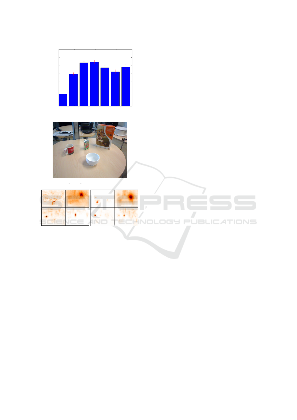
Figure 2: Performance of the individual features.
(a) table small 1: Bowl (I), cereal box
(II), coffee mug (III), soda can (IV)
I II
III IV
(b) Initial version
I II
III IV
(c) Extended version
Figure 3: Hough voting spaces of an exemple frame.
a lot, while recall did only slightly. The high-
confident false positives vanished.
7. Point Feature Histogram. Similar to HONV and
principal curvature, the support sizes of the PFH
and the normal computation were determined em-
pirically and set to 200 and 100 nearest neigh-
bours, while the histogram size was set to 7.
The PFH’s detection performance is similar to the
principal curvature (+29%), but with different re-
sults for the individual objects as depicted in Fig-
ure 1(g). While all others improved, the coffee
mug lost 10%.
For the fixed parameter set (patch size, tree depth,
etc.), the Depth HoG performs best among the tested
features (see Figure 2). It improves the detection
performance by approximately 34% and boosted in-
dividual as well as overall class purity. In contrast
to most other features, no object lost any of its de-
tection performance compared to the baseline. The
scaled depth value achieved similar results and is only
slightly worse. However, its power does not come
from its ability to describe the surface in a distinctive
fashion. It is rather a verification feature, that con-
tains the physical relationship of depth and scale, and
thus mainly rules out physically impossible object lo-
cations in scale space.
Features that operate on surface normals are
mostly outperformed by depth-map features. While
the latter is based on neighbours defined by the spa-
tial distances in image coordinates, the first are com-
puted from points in 3D space, which should result in
a more reliable information. The Hough Forest intrin-
sic split statistics indicate a higher noise ratio of the
surface normal features, which might explain this dis-
crepancy. Neither different normal calculation meth-
ods, scale space changes, smoothing mechanisms or
hole-filling methods, nor different feature scalings
and transformations improved the performance be-
yond the presented results.
Despite the overall increased detection perfor-
mance by combining RGB with depth features, the
time complexity of the corresponding calculations has
to be taken into account. There are GPU implemen-
tations available for all investigated algorithms, but
some of them are still in their beta phase and not yet
released as stable version. As a consequence, the
detection performance of GPU versions for princi-
pal curvature and FPFH either falls behind their CPU
counterparts (which are presented here), or the input
data is restricted to a special kind of point cloud that
is different from the data of the application scenario.
For those reasons, the scaled depth value, the So-
bel derivatives, and the Depth HoG are combined with
the RGB features to form the final feature vector. This
mixture sets the detection performance to 0.834AUC,
which is a jump of 46%. As depicted in Figure 1(h),
all strong false negatives disappeared and a precision
of more than 0.9 until a recall of 0.65 (coffee mug)
resp. 0.8 (all others) is achieved. The Hough space
in Figure 3(c) shows that the ambiguity between bowl
and coffee mug almost disappeared and there is less
clutter compared to the baseline (Figure 3(b)).
5 TIME COMPLEXITY AND
ADJUSTMENTS
The original Hough Forest implementation, with pa-
rameters set as in the feature evaluation, takes about
53 seconds on the target system for one single frame.
A household robot with this kind of detector would be
a real test of user patience.
The changes in run time reported in the follow-
Near Real-time Object Detection in RGBD Data
183

ing are not cummulative but are always given rela-
tive to the baseline implementation. A final evalua-
tion with respect to time and accuracy based on the
selected features and all changes to decrease the com-
putational complexity is given in Section 6.
5.1 Data and Dimensionality Reduction
Of the many parameters that have an impact on the
execution time the resolution of the image and the
number of scales (e.g. of the Hough voting space)
are especially crucial. The same general setting as
above was chosen during the following experiments,
while the scaled depth value and the depth derivatives
are used as depth features. The performance evalua-
tion is based on the average of five runs. The results
are reported in terms of AUC, while the time mea-
surements refer to wall time on the target system (an
octo-core Intel
R
Core
TM
i7-3770 CPU and a Nvidia
R
Titan
TM
Black GPU).
5.1.1 Image Resolution
The original resolution of the images is 640 × 320,
which is downsized at the beginning of the process-
ing pipeline. Affected parameters (e.g. support size of
the features, the patch size, and the smoothing param-
eters of the voting space) are adjusted accordingly.
Training and detection are computed on those down-
sized images, while the detection results, i.e. position,
scale, and bounding box, are upsized to the original
size. This does not only compress information of the
query image, but also the voting space.
The best compromise of time saving and decrease
of detection performance was found by grid search at
a scale of 0.5. The detection time decreased from 56s
to 14s (-75%), while the detection performance even
gained 3%. The performance increase is most prob-
ably caused by the implicit change of the RGB fea-
ture’s support size and noise suppression. Stronger
downscaling decreased the performance almost expo-
nentially.
5.1.2 Depth Normalization
In absence of depth data, the scale space is needed to
detect objects at distances that are different from the
ones learnt. From depth data, however, the correct
scale can be derived easily. We depth-normalize the
two points of the binary test functions of the Hough
Forest as well as the patch-object offset vectors. Since
the bounding boxes are generated by backprojection
(see Section 2), this depth normalized binary test
and voting also renders the need for multiple Hough
spaces over scale obsolete, which further reduces the
desk_2 table_small_1 table_small_2
70
80
90
100
110
120
mean p/r AUC and SEM in %
baseline
single scale
depth normalized
Figure 4: Depth normalization. Single scale and depth nor-
malization results normalized to the baseline performance.
complexity. Note, however, that the support size of
the feature computation stays uneffected.
Since the table small 1 dataset does not contain
much scale variance, the desk 2 and table small 2
datasets are used additionally. Figure 4 shows the
performance of the depth normalization compared to
the baseline performance (using five scales) and to the
performance using only the original scale (1.0).
The general observation from the three test sets
is that the mean performance does not suffer much
if depth normalization is applied. The performance
is even increased by 12% in the desk 2 dataset. Its
effects are different for the different objects. While
most improved, some suffer from a recall loss that is
comparable to using only one single scale. However,
the risk of a decreased detection performance is com-
pensated by the time savings (-77%).
5.1.3 Patch Offset
The detection mechanism of the Hough Forest can
be regarded as a classical sliding window approach,
in which every region of the query image is investi-
gated (in contrast to, for instance, interest point based
methods, where only a subsample of the whole im-
age is examined deeply). Since overlapping image
regions share information, it is redundant to exam-
ine two highly overlapping patches. The original im-
plementation of the Hough Forest does not take this
into consideration, but visits every single patch. Fig-
ure 5 shows the impact of different offsets on detec-
tion performance and time complexity by illustrating
the relationship between time saving, offset and per-
formance decrease, measured percental in compari-
son to the original offset of one pixel. A window off-
set of 2 already reduces the time complexity of the
classification and voting (not of the whole pipeline)
by about 70% while suffering a loss in performance of
only 1%. The influence on the whole pipeline heavily
depends on scale space and image resolution. With
VISAPP 2017 - International Conference on Computer Vision Theory and Applications
184

1
2 3
4 5
6
-100
-80
-60
-40
-20
0
execution time in %
-7
-6
-5
-4
-3
-2
-1
0
p/r AUC in %
Figure 5: Performance and time saving for different slid-
ing window offsets. A larger offset decreases performance
exponentially, but time saving only logarithmically.
the original pipeline and an offset of two pixel, about
20s are retrieved (-40%).
5.2 Parallel Processing
5.2.1 GPU Algorithms
Although the computation of the selected features is
very fast compared to other parts of the (original)
pipeline, their influence grows with the measures of
Section 5.1. All feature operators are replaced by
available GPU implementations if they did not de-
grade the overall detection performance. The mini-
mum and maximum filtration is replaced by equiva-
lent GPU erosion and dilation implementations.
With these changes, the feature computation is
35% faster, saving approximately 2 seconds from the
whole pipeline (-4%). The extraction of object hy-
potheses from the Hough space are ported to the GPU,
which further reduces the execution time of the whole
pipeline by another 4 seconds (-7%).
5.2.2 Multithreading
The target system’s multicore architecture is utilized
which allows parallel processing for most parts of the
detection pipeline. The run time decreases almost lin-
early with the number of cores. With five parallel
threads (and none of the other changes of this sec-
tion active) the detection finishes after approximately
11 seconds (-75%).
6 FINAL EVALUATION
The presented methods to increase performance (e.g.
different depth features) and decrease computation
time (e.g. depth normalization and subsampling) are
not independent of each other. The best combination
of the evaluated measures was tested empirically. The
desk_1
desk_2
desk_3
table_1
table_small_1
table_small_2
0.0
0.2
0.4
0.6
0.8
1.0
mean p/r AUC and SEM in %
HF
LINEMOD
DHF
Figure 6: Final results.
final solution uses the feature vector of Section 4, re-
sizes the input images with a factor of 0.7, applies
depth normalization and uses GPU calls as well as
multithreading. All parameters concerning spatial re-
lations were adapted according to the resizing opera-
tion while the patch size was set to 10 × 10 pixel.
A direct comparison to many of the state-of-the-
art methods (such as (Lai et al., 2011a; Bo et al.,
2013; Lai et al., 2011b)) is difficult, since most of
them fail to explicitly state their evaluation setup and
performance measure, to clarify the exact train and
test data, or to publish their software. In this section,
the proposed enhanced Hough Forest is compared to
its original RGB version (Gall et al., 2012) and to
LINEMOD (Hinterstoisser et al., 2011).
The general evaluation setup of Section 4 is now
used with all six test sets. LINEMOD is trained with
the same input data as the other methods (apart from
background data). The individual training images are
filtered with the foreground masks provided by the
database. The parameters of LINEMOD have been
optimized empirically for a fair comparison.
Figure 6 shows, that the enhanced Hough For-
est outperforms both reference methods by far.
LINEMOD produces a massive amount of false posi-
tives, which result in a low precision for most objects,
but also the recall statistics show major disadvantages
compared to the enhanced Hough Forest.
In terms of execution time, LINEMOD falls be-
hind as well. The used multi-scale variant needs ap-
proximately four seconds for each object, whereas the
optimized Hough Forest takes two seconds in total
and scales sub-linearly with the number of objects.
7 CONCLUSION AND FUTURE
WORK
The original implementation of the Hough Forest
from (Gall et al., 2012) is enhanced with depth data
Near Real-time Object Detection in RGBD Data
185

to improve both, its object detection performance as
well as runtime. By exploiting fast and descriptive
depth features, data reduction, as well as parallel pro-
cessing, the final implementation runs in near real-
time and can compete with state-of-the-art methods.
The output of the current detector are two-
dimensional axis-aligned bounding boxes in the im-
age coordinate system. To retrieve the full six degree
of freedom pose, the next step is to extract the region
in the point cloud that corresponds to the bounding
box and run ICP (Rusinkiewicz and Levoy, 2001) be-
tween a (learnt) 3D model of the object and the point
cloud region. Time complexity and result of ICP are
often improved by providing a good initial transfor-
mation, which could be generated by the Hough For-
est. To this aim the 2D Hough voting scheme needs to
be extended to 3D, in which object hypotheses are ac-
cumulated in real world and not in image coordinates.
REFERENCES
Arbeiter, G., Fuchs, S., Bormann, R., Fischer, J., and Verl,
A. (2012). Evaluation of 3d feature descriptors for
classification of surface geometries in point clouds. In
IROS 2012, pages 1644–1650.
Badami, I., St
¨
uckler, J., and Behnke, S. (2013). Depth-
enhanced hough forests for object-class detection and
continuous pose estimation. In SPME 2013, pages
1168–1174.
Ballard, D. (1981). Generalizing the hough transform to de-
tect arbitrary shapes. Pattern Recognition, 13(2):111–
122.
Bo, L., Ren, X., and Fox, D. (2013). Unsupervised feature
learning for rgb-d based object recognition. In Inter-
national Symposium on Experimental Robotics, pages
387–402.
Bo, L., Ren, X., and Fox, D. (2014). Learning hierarchical
sparse features for RGB-(D) object recognition. I. J.
Robotics Res., 33(4):581–599.
Breiman, L. (2001). Random forests. Machine Learning,
45(1):5–32.
Couprie, C., Farabet, C., Najman, L., and LeCun, Y. (2013).
Indoor semantic segmentation using depth informa-
tion. CoRR.
Farabet, C., Couprie, C., Najman, L., and LeCun, Y.
(2013). Learning hierarchical features for scene la-
beling. IEEE Transactions on Pattern Analysis and
Machine Intelligence, 35(8):1915–1929.
Gall, J., Razavi, N., and Van Gool, L. (2012). An introduc-
tion to random forests for multi-class object detection.
In Outdoor and Large-Scale Real-World Scene Anal-
ysis, pages 243–263.
Gupta, S., Girshick, R., Arbelaez, P., and Malik, J. (2014).
Learning rich features from RGB-D images for object
detection and segmentation. In ECCV 2014.
Hinterstoisser, S., Holzer, S., Cagniart, C., Ilic, S., Kono-
lige, K., Navab, N., and Lepetit, V. (2011). Multi-
modal templates for real-time detection of texture-less
objects in heavily cluttered scenes. In ICCV 2011,
pages 858–865.
Hinterstoisser, S., Lepetit, V., Ilic, S., Fua, P., and Navab,
N. (2010). Dominant orientation templates for real-
time detection of texture-less objects. In CVPR 2010,
pages 2257–2264.
Hinterstoisser, S., Lepetit, V., Ilic, S., Holzer, S., Bradski,
G., Konolige, K., and Navab, N. (2013). Model based
training, detection and pose estimation of texture-less
3d objects in heavily cluttered scenes. In ACCV 2012,
pages 548–562.
Janoch, A., Karayev, S., Jia, Y., Barron, J., Fritz, M.,
Saenko, K., and Darrell, T. (2011). A category-level
3-d object dataset: Putting the kinect to work. In ICCV
2011, pages 1168–1174.
Knopp, J., Prasad, M., Willems, G., Timofte, R., and
Van Gool, L. (2010). Hough transform and 3d surf
for robust three dimensional classification. In ECCV
2010, pages 589–602.
Lai, K., Bo, L., Ren, X., and Fox, D. (2011a). A large-scale
hierarchical multi-view rgb-d object dataset. In ICRA,
pages 1817–1824. IEEE.
Lai, K., Bo, L., Ren, X., and Fox, D. (2011b). A scalable
tree-based approach for joint object and pose recogni-
tion. In AAAI 2011.
Leibe, B., Leonardis, A., and Schiele, B. (2006). An im-
plicit shape model for combined object categorization
and segmentation. In Toward Category-Level Object
Recognition, pages 508–524.
M
¨
orwald, T., Prankl, J., Richtsfeld, A., Zillich, M., and
Vincze, M. (2010). BLORT - The Blocks World
Robotic Vision Toolbox. In Best Practice in 3D Per-
ception and Modeling for Mobile Manipulation (in
conjunction with ICRA 2010).
Rios-Cabrera, R. and Tuytelaars, T. (2013). Discrimina-
tively trained templates for 3d object detection: A real
time scalable approach. In ICCV 2013, pages 2048–
2055.
Rusinkiewicz, S. and Levoy, M. (2001). Efficient variants
of the icp algorithm. In International Conference on
3-D Digital Imaging and Modeling.
Rusu, R., Blodow, N., and Beetz, M. (2009). Fast point
feature histograms (fpfh) for 3d registration. In ICRA
2009, pages 3212–3217.
Rusu, R., Bradski, G., Thibaux, R., and Hsu, J. (2010). Fast
3d recognition and pose using the viewpoint feature
histogram. In IROS 2010, pages 2155–2162.
Tang, S., Wang, X., Lv, X., Han, T. X., Keller, J., He,
Z., Skubic, M., and Lao, S. (2013). Histogram of
oriented normal vectors for object recognition with a
depth sensor. In ACCV 2012, pages 525–538.
Tombari, F. and Di Stefano, L. (2010). Object recognition in
3d scenes with occlusions and clutter by hough voting.
In PSIVT 2010, pages 349–355.
Vergnaud, D. (2011). Efficient and secure generalized
pattern matching via fast fourier transform. In
AFRICACRYPT 2011, pages 41–58, Berlin, Heidel-
berg. Springer-Verlag.
Wang, W., Chen, L., Chen, D., Li, S., and Kuhnlenz, K.
(2013). Fast object recognition and 6d pose estimation
using viewpoint oriented color-shape histogram. In
ICME, pages 1–6.
VISAPP 2017 - International Conference on Computer Vision Theory and Applications
186
