An Efﬁcient Geometric Algorithm for Clipping and Capping Solid

Triangle Meshes

Aaron Scherzinger, Tobias Brix and Klaus H. Hinrichs

Department of Computer Science, University of M

unster, M

unster, Germany

Keywords:

Clipping, Two-Manifold Triangle Meshes, Geometry Processing.

Abstract:

Clipping three-dimensional geometry by arbitrarily oriented planes is a common operation in computer graph-

ics and visualization applications. In most cases, the geometry used in those applications is provided as surface

models consisting of triangles which are called meshes. Clipping such surface models by a plane cuts them

open, destroying the illusion of a solid object. Often this is not desirable, and the resulting mesh should

again be a closed surface model, e.g., when generating cross-sections in technical visualization applications.

We propose an algorithm which performs the clipping operation geometrically for a given input mesh on the

GPU. The intersection edges of the mesh and the clipping plane are then transferred to the CPU, where a cap

geometry closing the mesh is computed and eventually added to the clipped mesh. Our algorithm can process

solid (i.e., closed two-manifold) triangle meshes, or sets of non-intersecting solids, and has a worst-case run-

time of O(N + nlogn) where N is the number of triangles in the input geometry, and n is the number of input

triangles intersecting the clipping plane.

1 INTRODUCTION

In computer graphics and visualization, applying clip-

ping planes to a given geometry is a standard oper-

ation. It is usually implemented in rendering sys-

tems and application programming interfaces (APIs),

as clipping geometric objects against the planes of a

viewing frustum is essential for the rasterization pro-

cess. However, for some applications it is desirable to

provide the option of performing additional clipping

operations with user-deﬁned clipping planes. For in-

stance, such functionality is required in technical vi-

sualization like computer-aided design (CAD), or in

medical visualization. Moreover, these application

domains often require interactive frame rates, allow-

ing the user to modify the parameters of the plane in

real-time, while generating high-quality images.

Usually, the geometry used in computer graphics

applications is provided as surface models composed

of triangles which are called meshes. Such meshes

are restricted to surface representations and thus do

not contain any information about the interior of an

object. Clipping such surface models by a plane cuts

them open, and although it might be intentional in

some cases to obtain an open geometry, for several ap-

plication domains it is desirable to maintain the illu-

sion of a solid object, which requires closing the mesh

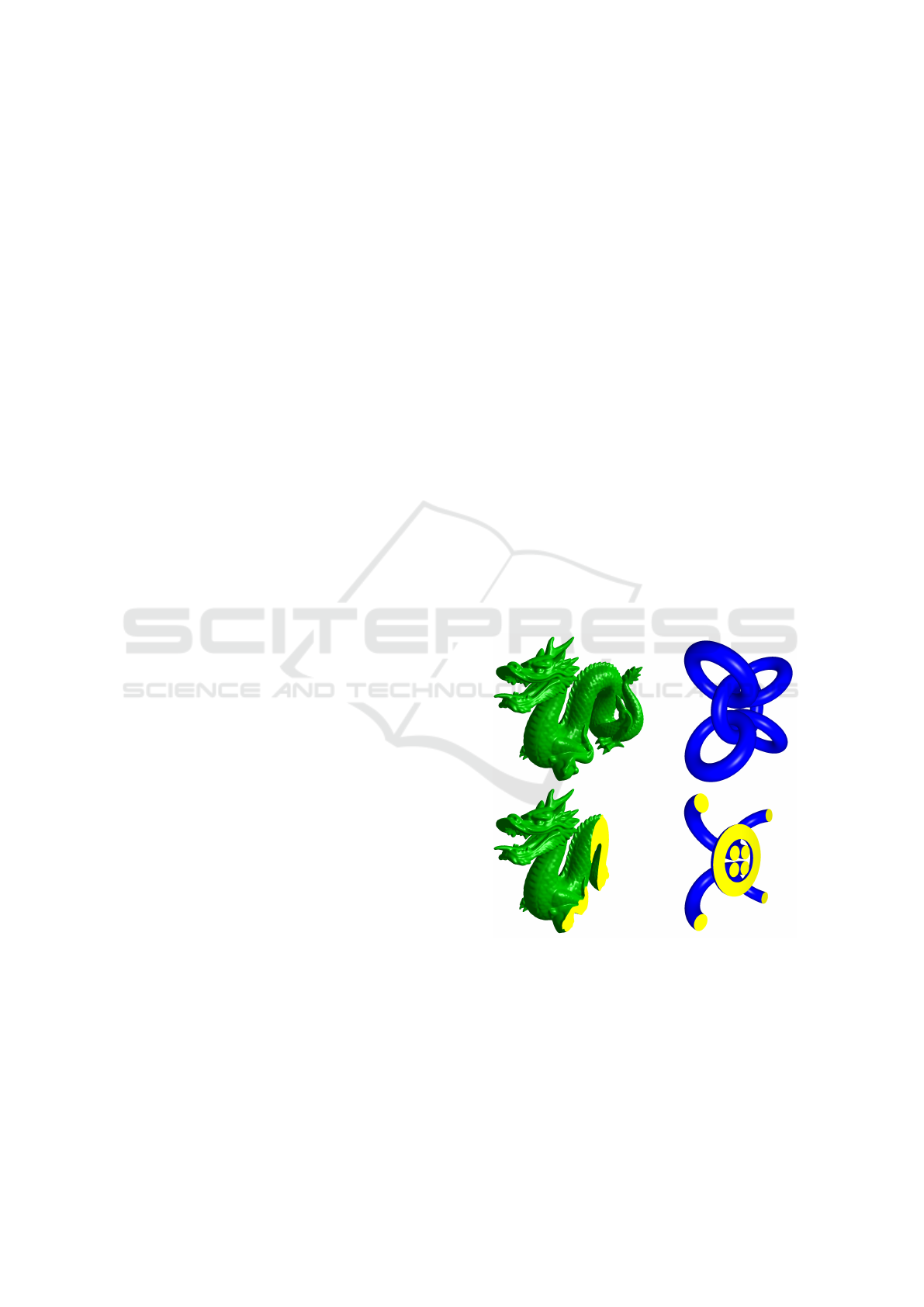
Figure 1: Example of solid-clipping the Stanford dragon

(left) and a test mesh consisting of several tori (right). In

both cases, the closing geometry is highlighted in yellow.

after performing the clipping operation. Especially

in CAD applications, this is a common requirement

when producing cross-sections of solid geometric ob-

jects to resolve spatial occlusion, allowing to examine

the internal structures of assemblies. This process is

referred to as solid-clipping (see Fig. 1). However,

Scherzinger A., Brix T. and H. Hinrichs K.

An Efﬁcient Geometric Algorithm for Clipping and Capping Solid Triangle Meshes.

DOI: 10.5220/0006097201870194

In Proceedings of the 12th International Joint Conference on Computer Vision, Imaging and Computer Graphics Theory and Applications (VISIGRAPP 2017), pages 187-194

ISBN: 978-989-758-224-0

187

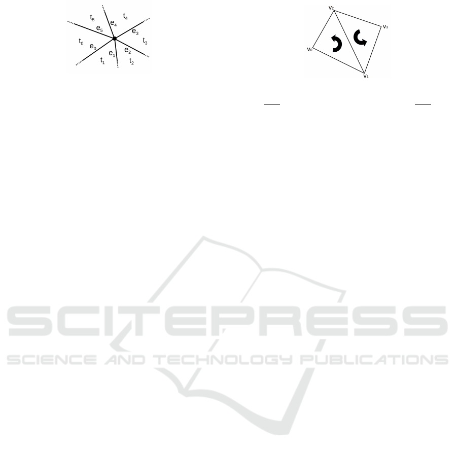
Figure 2: In a closed two-manifold triangle mesh, the trian-

gles incident to a vertex form a closed triangle fan and can

be arranged in a cyclic order.

closing a model after performing the clipping opera-

tion requires special effort, as additional faces have to

be created and rendered, and the methods for achiev-

ing this are usually not general, requiring speciﬁc data

structures and sophisticated algorithms.

In this paper, we propose an algorithm which

performs the solid-clipping process geometrically for

input meshes that are closed two-manifold triangle

meshes (see Sec. 2). Our algorithm performs the clip-

ping of the input mesh on the GPU. The intersecting

edges between the triangles of the mesh and the clip-

ping plane are then transferred to the CPU, while the

clipped mesh can be kept in graphics memory. From

the set of edges, a cap mesh is computed on the CPU

which closes the clipped mesh. Possible applications

of the algorithm include clipping of meshes for stere-

olithography, CAD applications, and isosurfaces ex-

tracted from volumetric data sets, where Lewiner et

al. (Lewiner et al., 2003) have proposed an extension

to the marching cubes algorithm to guarantee topo-

logical consistency for the resulting surface.

2 FUNDAMENTAL NOTIONS

This section includes some fundamental notions

which will be required in the remainder of the paper.

Deﬁnition 1 (Closed Two-Manifold Triangle Mesh).

A ﬁnite triangle mesh is called a closed two-manifold

triangle mesh if every edge of the mesh is shared be-

tween exactly two of its triangles, and if for every

vertex of the mesh the triangles incident to the ver-

tex form a closed fan, i.e., the edges e

and trian-

gles t

incident to the vertex can be arranged in a

cyclic order t

, e

, . . . ,t

n−1

, e

n−1

without repeti-

tions such that edge e

is shared between t

and t

i+1

(indices taken mod n). Other than in shared vertices

or edges, there is no intersection of triangles in the

mesh. A triangle mesh that is a closed two-manifold

is also called solid.

An example of the triangle and edge arrangement

around a vertex in Def. 1 is depicted in Fig. 2. In

addition to the constraints given in Def. 1, we assume

Figure 3: The two CCW triangles (v

, v

) and (v

, v

)

are consistently oriented, since the shared edge has orien-

tation v

in the ﬁrst triangle and orientation v

in the

second triangle.

that the triangles in the mesh are consistently oriented,

which we will deﬁne as follows.

Deﬁnition 2 (Consistently Oriented Triangle Mesh).

A triangle mesh is called consistently oriented if two

triangles sharing an edge induce opposite directions

on the shared edge.

As a convention, we will assume that the orienta-

tion of each triangle is chosen so that its vertices are

ordered counter-clockwise (CCW) with respect to the

triangle’s front face normal vector, i.e., the direction

of the surface normal of a triangle (v

, v

) is given

by the cross product (v

−v

)×(v

−v

). An example

of a consistent orientation is depicted in Fig. 3.

It should be noted that the deﬁnition above allows

meshes to consist of multiple unconnected compo-

nents, where some may constitute holes or hollows

within a solid object. While our algorithm is in-

herently able to handle such cases, we assume that

the orientation of the triangles is consistent with the

surface normals when constituting holes and exclude

cases where this condition is not fulﬁlled (which

would contradict the intuition of modeling solid ob-

jects, since an interior surface representing a hole

would have an outwards normal). An example would

be a solid sphere within a larger solid sphere where

the surface normals of both spheres point to the same

outward direction, which is depicted in Fig. 4(a). This

additional constraint can be formalized as follows.

Deﬁnition 3 (Solid Triangle Mesh Constraint).

For each ray R which intersects a consistently ori-

ented two-manifold triangle mesh M holds that it is

either a degenerate case, i.e., R intersects at least one

edge or vertex of a triangle of M, or the set of trian-

gles of M that are intersected by R and ordered along

the direction of R are given by t

, . . . ,t

so that for

each triangle t

, i = 2 · m, the angle between the direc-

tion vector of the ray d

and the triangle’s normal n

is greater than 90

◦

, i.e., d

· n

< 0, while for each tri-

angle t

, j = 2 · m + 1, the angle is less than 90

◦

, i.e.,

· n

> 0.

Intuitively, the above constraint corresponds to the

idea that a ray intersecting the geometry will alternate

GRAPP 2017 - International Conference on Computer Graphics Theory and Applications

188

(a) Example of two solids

stacked into each other.

The surface normals are

depicted by arrows.

(b) A ray intersecting a

solid alternates between

being outside of the solid

and within the solid.

Figure 4: Solid modeling constraints.

between being outside of the solid and being inside

the solid each time it intersects the surface given by

the triangles of the mesh (see Fig. 4(b)). If this as-

sumption holds, cases such as in Fig. 4(a) can also

be handled by the algorithm when introducing an ad-

ditional processing step without changing the overall

asymptotic runtime (see Sec. 4.4).

3 RELATED WORK

Several approaches to realize solid-clipping have been

proposed. Probably the most common method is

an image-based technique which utilizes the stencil

buffer of the graphics hardware to render additional

geometry, thus conveying the impression of solid ob-

jects (McReynolds and Blythe, 2005). This approach

is often referred to as capping, and the geometric ob-

jects embedded in the clipping plane which are ren-

dered additionally to close the mesh are called cap

polygons. For technical visualization, other image-

based techniques have been proposed, such as the in-

teractive view-dependent cutaway rendering by Burns

and Finkelstein (Burns and Finkelstein, 2008). Trapp

and D

ollner (Trapp and D

ollner, 2013) have proposed

a technique which allows the use of more complex

clipping surfaces by applying an offset map to the

plane. Despite the fact that capping techniques allow

to efﬁciently render images of the clipped objects, a

general drawback is that they only construct the cap

polygons in image space and do not allow to retrieve

a clipped and closed version of the surface model for

further geometric computations.

An alternative approach which solves the prob-

lem of solid-clipping geometrically is the use of con-

structive solid geometry (CSG), which provides a set

of operations on boundary representations (b-reps) of

the geometry (Foley et al., 1996). While providing a

ﬂexible and general toolbox for geometry processing,

those methods often require a speciﬁc representation

of the geometric objects explicitly storing topological

information such as the winged-edge data structure or

similar representations.

Weiskopf et al. (Weiskopf et al., 2003) have pro-

posed a technique for interactive clipping of volumet-

ric data sets in texture-based volume rendering ap-

plications. Using volumetric representations of both

the input geometry and the clipping objects, voxel-

based methods provide a lot of ﬂexibility regarding

the shape of the clipping objects and allow to re-

trieve the new geometry after performing the clipping

process. Unfortunately, in order to apply these tech-

niques to a triangle mesh, they require the input mesh

to be converted to a voxel representation via a vox-

elization method such as the ones proposed in (Huang

et al., 1998) or (Schwarz and Seidel, 2010). Addition-

ally, if a surface model representation of the clipped

geometry is required afterwards for further process-

ing, the obtained voxel representation has to be con-

verted back again after performing the clipping.

Erleben and Henriksen (Erleben and Henriksen,

2006) have proposed a geometric algorithm for clip-

ping a solid mesh composed of convex faces and

closing the geometry afterwards. However, their ap-

proach requires an input mesh representation similar

to a half-edge data structure. Moreover, the runtime

of their algorithm is O(n

), which might be problem-

atic in real-time applications.

We propose a geometric algorithm for interac-

tively clipping solid triangle meshes and subsequently

closing these objects. The output of our algorithm

is again a solid triangle mesh which allows to store

or further process the geometry data after the solid-

clipping operation. Our algorithm does not need any

pre-processing phase to convert the input geometry to

a speciﬁc representation as the clipping is performed

on the individual triangles and solves the problem in

a worst-case runtime of O(N +nlog n) where N is the

number of triangles in the input geometry and n is the

number of triangles in the input geometry that actu-

ally intersect the clipping plane. Since the clipping is

performed in parallel on the GPU, the O(N) step can

be computed efﬁciently in practice.

4 PROPOSED ALGORITHM

4.1 Workﬂow

An overview of the workﬂow for our proposed

method is depicted in Fig. 5. First, the clipping of

the input mesh against a plane is performed in parallel

for each individual triangle on the GPU (see Sec. 4.2).

We use OpenGL’s transform feedback functionality to

An Efﬁcient Geometric Algorithm for Clipping and Capping Solid Triangle Meshes

189

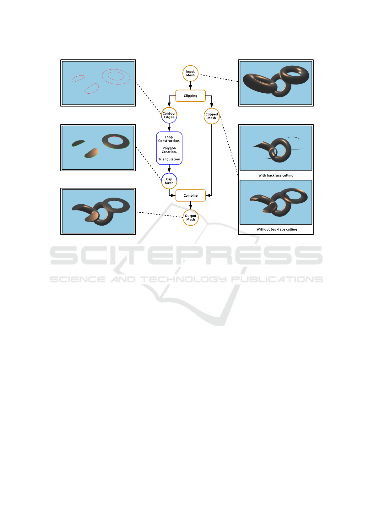
Figure 5: Workﬂow of our proposed algorithm. Boxes denote operations of the algorithm while circles correspond to meshes,

which are illustrated by the rendered examples. Operations and data on the GPU are depicted using the orange color while

operations and data on the CPU are depicted in blue. Circles with both colors denote data transfer between CPU and GPU.

retrieve both the clipped mesh as well as the intersec-

tion geometry of the mesh and the clipping plane into

separate buffers. The intersection corresponds to a set

of contour edges which are downloaded to the CPU

for creating the cap mesh while the clipped version of

the input mesh is kept on the GPU.

From the (unordered) set of edges, we then con-

struct a set of loops, i.e., closed polygonal chains

which describe the boundaries of polygonal regions

embedded in the clipping plane (see Sec. 4.3). De-

pending on its orientation, each loop may constitute

either the outer boundary of a polygon or a hole within

such a polygon. In the next step, a hierarchy of the

loops is computed which is then traversed to com-

pute the actual set of polygons (potentially contain-

ing holes) which correspond to the planar geometry

necessary to close the clipped input mesh and thus

correspond to the capping polygons (see Sec. 4.4).

Afterwards, a triangulation of those polygons is per-

formed to construct the actual triangle cap mesh (see

Sec. 4.5). This mesh can then be transferred to GPU

memory and closes the clipped input mesh, so that

their combination constitutes the solid-clipped mesh

which again is a solid triangle mesh. Examples of the

geometries resulting from the different stages of the

workﬂow are depicted in Fig. 5.

4.2 Clipping

Clipping a triangle against a plane with the normal

n = (n

, n

= 1, and (signed) distance d from

the origin computes the intersection of the triangle

with the half-space (x, y, z) · n − d > 0 bounded by the

clipping plane, which can either be the empty set, a

triangle, or a quadrilateral (which can be decomposed

into two triangles). It should be noted that we deﬁne

the half-space as being strictly positive which avoids

special cases like triangles lying exactly in the clip-

ping plane or the existence of degenerated triangles

after the clipping operation.

We assume that an input mesh is given as a GPU

representation for rendering, e.g., an OpenGL buffer

object, and compute the intersection of the triangle

and the positive half-space using a geometry shader.

The implementation relies on the GPU triangle clip-

ping method proposed by McGuire in (McGuire,

2011), which is based on an algorithm proposed by

Sutherland and Hodgman (Sutherland and Hodgman,

1974). For triangles, their method can be reduced to a

few speciﬁc cases which are depicted in Fig. 6. Trian-

gles can either be discarded or completely retained, or

have to be clipped against the plane (cases (3) and (4)

in Fig. 6). When clipping a triangle, two vertices v

GRAPP 2017 - International Conference on Computer Graphics Theory and Applications

190

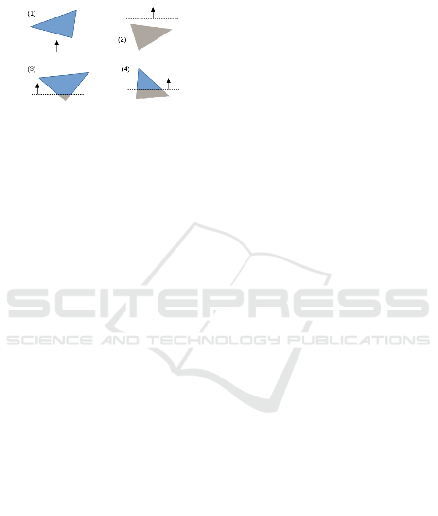
Figure 6: Examples of the four cases that may occur when

a triangle is clipped against a plane. In case (1), the whole

triangle is retained, while in case (2), it is completely dis-

carded. In the other two cases the triangle is actually

clipped, resulting in a quadrilateral in case (3) and in a tri-

angle in case (4). The arrow represents the direction of the

plane normal.

and v

corresponding to the intersection of two edges

of the triangle and the clipping plane are computed

using linear interpolation along the triangle’s edges to

construct either a quadrilateral or a triangle. For the

actual shader code, we refer to the triangle clipping

listing in McGuire’s paper. When clipping a trian-

gle, we linearly interpolate the vertex attributes such

as colors, normals, or texture coordinates between the

original vertices in the same way as the vertex posi-

tions. If the clipping operation yields a quadrilateral

(case (3) in Fig. 6), we decompose it into two triangles

with consistent orientation. As stated above, degener-

ated triangles are avoided by the convention of using

the strictly positive half-space.

When a triangle is clipped against the plane, the

two vertices v

and v

form an edge which is em-

bedded in the clipping plane and corresponds to the

intersection of the plane and the triangle. The geome-

try shader writes those edges and the clipped triangles

into different output streams, storing the clipped mesh

and the intersection edges in separate buffer objects.

While we retain the original orientation of the clipped

triangles, we invert the direction of the intersection

edges so that a polygon constructed from those edges

is consistently oriented to the clipped input mesh.

Since we compute the clipping operation on the

GPU, the triangles can be processed very efﬁciently in

parallel. However, if the mesh is not already present

on the GPU or should not be uploaded for later ren-

dering, the clipping can also be performed on the CPU

by processing the individual triangles sequentially in

O(N) time. It should be noted that a trivial upper

bound for the number n of triangles that intersect the

plane, which corresponds to the number of intersec-

tion edges, is O(N), although in practice the num-

ber of edges is usually much smaller than the overall

number of triangles N.

4.3 Loop Construction

After performing the GPU clipping operation, we

download the intersection edges to the CPU while

keeping the triangles of the clipped mesh in graph-

ics memory. Due to the parallelity of the clipping

operation and the potentially random order of trian-

gles in the input mesh, the list of edges is not given in

any speciﬁc order. For a closed two-manifold triangle

mesh, the set of intersection edges always constitutes

a set of closed loops for which is guaranteed that the

loops are not self-intersecting and that there are no

intersections between different loops.

Theorem 1.

The intersection of a plane P and a ﬁnite consistently

oriented closed two-manifold triangle mesh M is ei-

ther the empty set, or a ﬁnite set of edges embedded

in P, which form one or more closed loops without

self-intersections. No pair of two edges contained in

different loops intersects.

Proof. Let S be the set of edges that resulted from clip-

ping M against P. Since each edge s ∈ S is the inter-

section of a triangle T ∈ M and the plane P, it has to

be embedded in P, i.e., s ⊂ P. The rest of the proof

consists of two parts.

(i) For each clipping edge s = pq, s ∈ S, a successor

edge s

= qr, s

∈ S, can be found.

Let A = (v

, v

), A ∈ M, be a triangle for

which at least one of its vertices v ∈ {v

, v

}

lies in the positive half-space bounded by P, and

at least one of its vertices w ∈ {v

, v

}, w 6= v,

lies in the negative half-space. Then the inter-

section of P and A constitutes a line segment

s ∈ S, s = pq, where p and q are the intersec-

tions of two edges e, f of A and P. W.l.o.g. let q

be the intersection point of e and P.

Because of the characteristics of a consistently

oriented two-manifold triangle mesh, there ex-

ists exactly one triangle B ∈ M, B 6= A , which

shares the edge e with A. Then the intersection

of B and P also constitutes a line segment with

q as one of its endpoints. Because of the consis-

tent orientation, the edge e is inversely directed

in B compared to A and thus s

has to be directed

from q to a point r, i.e., s

= qr.

Since for each clipping edge s a successor s

can be

found and the mesh is ﬁnite, each edge is contained

in a closed loop. The second part of the proof now

considers the intersections between line segments.

(ii) Except for two consecutive edges in a loop,

which intersect in their common endpoint, no

pair of two edges e, f ∈ S, e 6= f , intersect.

An Efﬁcient Geometric Algorithm for Clipping and Capping Solid Triangle Meshes

191

Each edge s ∈ S is the intersection of a trian-

gle T ∈ M and P, which implies s ⊆ T . Let

A, B ∈ M, A 6= B be two triangles that intersect

the plane, and let e, f ∈ S, e 6= f be the two cor-

responding intersection edges with the plane P.

Then e ∩ f 6=

0 ⇒ A ∩ B 6=

0, and if this is true,

one of two cases has to apply:

(1) A and B share a common edge, which inter-

sects P as in (i), and e and f are consecutive

edges of a loop. X

(2) M is not a two-manifold triangle mesh, as it

is self-intersecting.

Since no pair of line segments is intersecting, except

for the consecutive edges of a loop, and every edge is

contained in a closed loop, Thm. 1 is correct.



It should be noted that the orientation of the re-

sulting loops is consistent with the mesh, meaning

that a loop is CCW regarding the inverted normal of

the clipping plane, i.e., the actual surface normal of

the resulting cap polygon, if it constitutes the outer

boundary of a polygon, and clockwise (CW) if it con-

stitutes a hole. This follows directly from the con-

vention we have chosen for the triangle orientation of

the consistently oriented mesh, and the fact that the

orientation of the edges retrieved from the clipping

process is consistent with the clipped triangles of the

input mesh. This property will be relevant for the sub-

sequent steps presented later on.

Now that the existence of loops in the set of edges,

and the membership of each edge in one of the loops,

has been established, the loop construction algorithm

will be outlined. Basically, the algorithm starts to cre-

ate a new loop by picking an arbitrary edge from the

set of contour edges. Afterwards, it searches for its

successor in the set of edges, i.e., for an edge that has

a start vertex with a position identical to that of the

end vertex of the current edge, and appends it to the

loop. If the end vertex of the new edge closes the loop,

the process is started again with one of the remaining

edges and a new loop. Otherwise, the new edge be-

comes the current edge, for which a successor has to

be found. The process is repeated until no edge is left

that is not already part of a loop. To reduce the search

time for a successor, in a ﬁrst step the algorithm sorts

the edges lexicographically in ascending order with

respect to the position of their start vertices. This al-

lows to perform binary search to ﬁnd an edge by its

start vertex position. Algorithm 1 shows the complete

loop construction procedure.

Since Thm. 1 states that the number of edges is

ﬁnite, each edge has a successor, and every loop is

closed, the algorithm eventually terminates, as it ex-

amines each edge exactly once before appending it to

Algorithm 1: Loop Construction.

Input: Vector<Edge> edges

Output: List<Loop> loops

LexicographicSortByStartPosition(edges)

while edges not empty do

Loop l = new empty Loop

Edge currentEdge = edges.front()

l.append(currentEdge.start)

edges.erase(currentEdge)

while currentEdge.end.position 6=

l.front().position do

Edge next =

ﬁndSuccessor(edges,currentEdge)

currentEdge = next

l.append(currentEdge.start)

edges.erase(currentEdge)

loops.append(l)

a loop and removing it from the input list. If the lex-

icographical sorting is implemented by inserting all

edges into a balanced tree (e.g., an AVL tree), the algo-

rithm has a worst case time complexity of O(mlog m)

for m input edges. This upper bound can be estab-

lished by analyzing the actions the algorithm takes for

each edge:

1. Each edge is selected by either using front

(which selects the ﬁrst edge in the list, i.e., left-

most element in the tree), or findSuccessor. In

an AVL tree, both of these operations can be exe-

cuted in O(logm) time.

2. Each edge is erased from the tree, which takes

O(logm) time.

3. Each edge is appended to the end of a list (i.e., the

current loop), which can be realized in O(1) time.

Since each edge is only handled once and is directly

erased from the tree afterwards, processing an edge

takes O(log m) time. All of the m edges are thus pro-

cessed in O(m logm) time. Inserting the edges into

the tree at the start also takes O(m logm) time. The

complete loop construction algorithm runs therefore

in O(mlog m) time. Since the number m of edges cor-

responds to the number n of triangles intersecting the

clipping plane, this can also be written as O(nlogn).

4.4 Polygon Creation

For convenience, we transform all of the edges, i.e.,

their vertices, into the xy-plane for the next two steps,

which allows us to perform the polygon creation and

triangulation steps in R

. This can be realized by a

rotation matrix which can be computed from the clip-

ping plane normal. Optionally, an additional trans-

lation and scaling of the vertices can be performed

GRAPP 2017 - International Conference on Computer Graphics Theory and Applications

192

Figure 7: The contour A corresponds to the outer boundary

of a polygon, while the contours B and C correspond to

holes in that polygon. The contour D is nested within a hole

and corresponds to a new polygon.

to normalize the coordinates. It should be noted that

along with the projected vertices, we retain the origi-

nal vertex positions in R

which will be used for the

output mesh to avoid numerical issues that might arise

from transforming the vertices back and forth.

Since some of the loops reconstructed from the set

of edges may constitute the outer contours of poly-

gons while others may correspond to holes within

those polygons, we need to compute the hierarchical

ordering of the loops, which is called polygon nest-

ing (see Fig. 7). Note that not all contours have to be

nested in a single hierarchy. Instead, there may exist

several trees like the one in the example, which form

a forest of trees. Such a forest always exists and the

hierarchical ordering is unambiguous, since no inter-

sections between two different loops exist. Each loop

is thus either the root of a tree or has a parent loop

which completely contains it. Moreover, each root

corresponds to the outer contour of a polygon, since

the outermost loop cannot constitute a hole.

Due to the characteristics of a consistently ori-

ented solid triangle mesh and the additional constraint

given in Def. 3, each contour at the root of a tree as

well as each contour with an even number of prede-

cessors has a CCW orientation and corresponds to the

outer boundary of a polygon, while each contour with

an uneven number of predecessors has a CW orienta-

tion and corresponds to a hole. This becomes appar-

ent when examining rays intersecting the geometry as

in Def. 3 which lie in the clipping plane. Each of those

rays alternates between the outside and the inside of

the solid each time it crosses one of the edges.

To efﬁciently compute the polygon nesting struc-

ture, we apply the algorithm proposed by Bajaj and

Dey (Bajaj and Dey, 1990). Their method computes

the hierarchy of the polygons in O(k + (l + r) log(l +

r)) where k is the number of input vertices of the poly-

gons, l is the number of polygons, and r is the num-

ber of reﬂex vertices, i.e., vertices with an inner an-

gle > 180

◦

, in the set of vertices. Since l and r are

much smaller than k, the algorithm runs faster than

O(k logk) in practice. It should be noted that the num-

ber k of vertices equals the number n of contour edges,

so that the runtime of the algorithm is in O(nlogn).

First, the algorithm breaks all of the loops

into subchains, i.e., it partitions each loop into x-

monotone sequences of vertices, which can be done in

O(k) time. These subchains are sorted lexicographi-

cally by their endpoints from left to right. The al-

gorithm then performs a plane sweep using a sweep

line L while maintaining the vertical ordering O of

the subchains induced by L. The sweep line stops at

each endpoint of a subchain and updates the ordering

O to determine the parent of each loop. The output

of the algorithm is a directed acyclic graph G which

contains a node for each loop L and corresponds to the

nesting structure of the contours. For details about the

algorithm, we refer the reader to the original paper by

Bajaj and Dey. After computing the nesting structure,

it can easily be traversed to extract each individual

polygon together with its holes. During this traver-

sal, an additional step could be integrated to correct

the orientation of inner loops corresponding to holes

when dealing with cases such as the one depicted in

Fig. 4(a) (see Sec. 2) by inverting the orientation of

the loops at each other level of the hierarchy, pro-

ducing an alternating CCW-CW order in the sequence

of levels of the nesting structure. This only requires

O(n) additional computation time and thus does not

change the overall runtime complexity.

4.5 Triangulation

Polygon triangulation is one of the fundamental prob-

lems in computational geometry. Chazelle was the

ﬁrst to propose a linear-time algorithm for triangu-

lation of simple polygons (Chazelle, 1991). How-

ever, his method does not seem to be applicable in

practice. Instead, usually one of several existing

O(k logk) (where k is the number of input vertices)

methods for polygon triangulation is applied. Here,

we use a two-step method which consists of partition-

ing the polygon into y-monotone pieces in O(k logk)

and afterwards triangulating each of the pieces in

O(k) time. The method to partition a polygon into

monotone pieces is due to Lee and Preparata (Lee and

Preparata, 1977) and the linear time algorithm for tri-

angulating a monotone polygon has been proposed by

Garey et al. (Garey et al., 1978). The complete algo-

rithm is summarized in (de Berg et al., 2008).

For the monotone partitioning of the input poly-

gon in the ﬁrst step, vertices are classiﬁed into various

types and sources of non-monotonicity are removed

by adding additional diagonals, splitting the polygon

into monotone pieces. The algorithm performs this

partitioning operation using a plane sweep which has

a runtime complexity of O(k log k), where k is the

number of input vertices. Afterwards, each monotone

An Efﬁcient Geometric Algorithm for Clipping and Capping Solid Triangle Meshes

193

polygon resulting from the previous step can be trian-

gulated in O(k) time by iterating over the vertices in

decreasing y-direction and connecting the left and the

right chain. The overall worst-case runtime of the tri-

angulation step is thus in O(k log k). Again, the num-

ber k of input vertices equals the number n of contour

edges, so that the runtime is in O(nlogn).

Since the orientation of the original edges is re-

tained during triangulation, the cap mesh is consis-

tently orientated with the clipped mesh. If the trian-

gulation is not consistently oriented in itself, this can

easily be corrected using an O(n) scan over the list

of triangles. Moreover, a simple runtime optimization

of the triangulation can be added by testing each poly-

gon for convexity and applying a very simple O(n) tri-

angulation for convex polygons instead of the afore-

mentioned algorithm. However, this does not change

the upper bound of the runtime complexity.

For the set of triangles resulting from the trian-

gulation, the original 3D positions of the vertices (as

computed during clipping) are used instead of the ver-

tex positions transformed into the xy-plane. If the

vertices contain normal vectors, the normal vector at-

tribute for all of the vertices in the cap mesh is set to

the inverted normal of the clipping plane, which cor-

responds to the normal vector of the cut surface. After

ﬁnishing the triangulation step for all polygons, the

cap mesh is complete. The output geometry is then

created by combining the cap mesh with the clipped

input mesh (e.g., by uploading the cap mesh to the

GPU). Since each contour edge of the cap mesh is

shared between a triangle of the clipped input mesh

and a triangle of the cap mesh, and the shared edges

induce opposite direction in the meshes due to the

output of the clipping step, the output mesh is a con-

sistently oriented closed two-manifold triangle mesh.

Since the runtime of the clipping step (if not per-

formed in parallel) is O(N) and each subsequent step

of the algorithm is in O(n logn) where n is the num-

ber of triangles intersecting the plane, the algorithm

has an overall worst case runtime of O(N + nlog n).

5 CONCLUSION AND FUTURE

WORK

We have proposed an efﬁcient method for geometri-

cally clipping and capping a closed two-manifold tri-

angle mesh in O(N + n logn). Our method performs

the clipping on the GPU and transfers the contour

edges to the CPU, where the cap mesh is computed to

close the clipped input mesh. One of the drawbacks of

our algorithm is the numerical stability, which might

be problematic particularly in the loop construction.

However, this can be mitigated by using a small ep-

silon as an allowed distance between the end vertex of

an edge and the start vertex of its successor. Another

problem of our method may be the quality of the tri-

angulation in the last step. In future work, we will try

to improve this step by applying constrained Delau-

nay triangulation or use of additional Steiner vertices

to increase the quality of the cap mesh.

REFERENCES

Bajaj, C. L. and Dey, T. K. (1990). Polygon nesting and

robustness. Inf. Proc. Lett., 35(1):23–32.

Burns, M. and Finkelstein, A. (2008). Adaptive cutaways

for comprehensible rendering of polygonal scenes.

ACM Transactions on Graphics, 27(5):154:1–154:7.

Chazelle, B. (1991). Triangulating a simple polygon in lin-

ear time. Discrete & Comput. Geom., 6(5):485–524.

de Berg, M., Cheong, O., van Kreveld, M., and Overmars,

M. (2008). Computational Geometry: Algorithms and

Applications. Springer, 3rd edition.

Erleben, K. and Henriksen, K. (2006). A simple plane

patcher algorithm. Technical Report DIKU-TR-

06/09, Department of Computer Science, University

of Copenhagen.

Foley, J. D., van Dam, A., Feiner, S. K., and Hughes, J. F.

(1996). Computer Graphics: Principles and Practice,

2nd ed. in C. Addison-Wesley.

Garey, M. R., Johnson, D. S., Preparata, F. P., and Tarjan,

R. E. (1978). Triangulating a simple polygon. Inf.

Proc. Let., 7(4):175–179.

Huang, J., Yagel, R., Filippov, V., and Kurzion, Y. (1998).

An accurate method for voxelizing polygon meshes.

In Proceedings of the 1998 IEEE Symposium on Vol-

ume Visualization, VVS ’98, pages 119–126. ACM.

Lee, D. T. and Preparata, F. P. (1977). Location of a point

in a planar subdivision and its applications. SIAM J.

on Computing, 6(3):594–606.

Lewiner, T., Lopes, H., Vieira, A. W., and Tavares, G.

(2003). Efﬁcient implementation of marching cubes’

cases with topological guarantees. J. of Graphics

Tools, 8:2003.

McGuire, M. (2011). Efﬁcient triangle and quadrilateral

clipping within shaders. J. of Graphics, GPU, and

Game Tools, 15(4):216–224.

McReynolds, T. and Blythe, D. (2005). Advanced Graphics

Programming Using OpenGL. Morgan Kaufmann.

Schwarz, M. and Seidel, H.-P. (2010). Fast parallel surface

and solid voxelization on gpus. ACM Transactions on

Graphics, 29(6):179:1–179:10.

Sutherland, I. E. and Hodgman, G. W. (1974). Reentrant

polygon clipping. Comm. of the ACM, 17(1):32–42.

Trapp, M. and D

ollner, J. (2013). 2.5d clip-surfaces for

technical visualization. J. of WSCG, 21(1):89–96.

Weiskopf, D., Engel, K., and Ertl, T. (2003). Interactive

clipping techniques for texture-based volume visual-

ization and volume shading. IEEE Transactions on

Visualization and Computer Graphics, 9(3):298–312.

GRAPP 2017 - International Conference on Computer Graphics Theory and Applications

194