
A Simple Node Ordering Method for the K2 Algorithm
based on the Factor Analysis
Vahid Rezaei Tabar
Department of Statistics, Faculty of mathematics and Computer Sciences, Allameh Tabataba'i University, Tehran, Iran
vhrezaei@atu.ac.ir
Keywords: Bayesian Network, Factor Analysis, K2 Algorithm, Node Ordering, Communality.
Abstract: In this paper, we use the Factor Analysis (FA) to determine the node ordering as an input for K2 algorithm
in the task of learning Bayesian network structure. For this purpose, we use the communality concept in
factor analysis. Communality indicates the proportion of each variable's variance that can be explained by
the retained factors. This method is much easier than ordering-based approaches which do explore the
ordering space. Because it depends only on the correlation matrix. As well, experimental results over
benchmark networks ‘Alarm’ and ‘Hailfinder’ show that our new method has higher accuracy and better
degree of data matching.
1 INTRODUCTION
Bayesian networks (BNs) are directed acyclic graphs
(DAGs), where the nodes are random variables, and
the arcs specify the conditional independence
structure between the random variables (Pearl, 1988;
Geiger, 1990; Jensen, 1996; Friedman, 1997). The
learning task in a BN can be separated into two
subtasks, structure learning; that is to identify the
topology of the network, and parameter learning;
that is to estimate the parameters (conditional
probabilities) for a given network topology
(Heckerman, 1994; Ghahramani, 1998; Grossman,
2004). While there are large collections of variables
in many applications, a fully BN approach for
learning structure upon variables can be expensive
and lead to high dimensional models (Friedman,
2000; Perrier, 2008). In other words, the number of
BN structures is super-exponential in the number of
random variables in the domain. To overcome such
difficulties in terms of computational complexity,
several approximations have been designed, such as
imposing a previous ordering on the domain
attributes or using other approaches trying to reduce
the state space of this problem (Spirtes, 1993;
Madigan, 1995). The K2 algorithm is one of the
basic methods for effectively resolving the above
problems (Cooper, 1992). This algorithm works with
a node ordering as an input. It starts by assuming
that a node lacks parents, after which in every step it
adds incrementally that parent whose addition most
increases the probability of the resulting structure.
K2 stops adding parents to the nodes when the
addition of a single parent cannot increase the
probability. As mentioned, the K2 algorithm
receives as input a total ordering of the variables
which can have a big influence on its result. Thus,
finding a good ordering of the variables is also
crucial for the algorithm success (Larranaga, 1996;
Ruiz, 2005; Lamma, 2005; Chen, 2008).
The K2 algorithm reduces this computational
complexity by requiring a prior ordering of nodes as
an input, from which the network structure will be
constructed.
Chow & Liu, (1968) proposed a method derived
from the maximum weight spanning tree algorithm
(MWST). This method associates a weight to each
edge. This weight can be either the mutual
information between the two variables or the score
variation when one node becomes a parent of the
other. When the weight matrix is created, a usual
MWST algorithm gives an undirected tree that can
be oriented given a chosen root. Based on the
Heckerman et al. (1994) propose, one can use the
oriented tree obtained with the maximum weight
spanning tree algorithm (MWST) to generate the
node ordering. The algorithm which uses the class
node as a root called "K2+T" (Leray et al., 2004).
Where the class node is the root node of the tree, the
class node can be interpreted as a cause instead of a
Tabar, V.
A Simple Node Ordering Method for the K2 Algorithm based on the Factor Analysis.
DOI: 10.5220/0006095702730280
In Proceedings of the 6th International Conference on Pattern Recognition Applications and Methods (ICPRAM 2017), pages 273-280
ISBN: 978-989-758-222-6
Copyright
c
2017 by SCITEPRESS – Science and Technology Publications, Lda. All rights reserved
273

consequence. That’s why Leray et al. (2004)
proposed the reverse order called "K2-T".
In general, node ordering algorithms are
categorized into two groups; evolutionary algorithms
and heuristic algorithms. Initial research on
evolutionary algorithms has provided extensive
experimental results through various crossover and
mutation methods (Romero, 1994; Larranaga 1996;
Hsu et al., 2007). In terms of heuristic methods,
Hruschka et al. (2007) introduced the feature
ranking-based node ordering algorithm, which is a
type of feature selection method in the classification
domain. It measures dependencies of variables over
the class label using
statistical tests and
information gain; it then sorts the variables by the
dependence-based scores. The sorted variables are
regarded as the node ordering. Chen et al. (2008)
incorporated information theory and exhaustive
search functions in their algorithm. The algorithm
comprises three major phases. In the first two
phases, it constructs an undirected structure through
mutual information, independence tests, and d-
separation. The last phase is related to determination
of node ordering.
In this paper, we focus on the factor analysis for
determining the node ordering as an input for K2
algorithm. The steps of our method are as follows:
First right number of factors must be
extracted.
Once the extraction of factors has been
completed, we use the "Communalities"
which tells us how much of the variance in
each of the original variables is explained
by the extracted factors. In other words,
communality is the proportion of each
variable's variance that can be explained by
the common factors.
We consider the communality as a novel
method for determining the node ordering
as an input for K2 algorithm.
Our novel method is much easier than ordering-
based approaches which do explore the ordering
space. To the best of our knowledge, the most
effective heuristic algorithm for determining the
node ordering is the one proposed by Chen et al.
(2008) whose time complexity is O(n
4
). However,
our methodology has less complexity compared to
other node ordering methods. Because our method
depends only on the correlation matrix.
The paper is organized as follows. First an
introduction to the Factor Analysis is presented. We
then introduce our methodology for learning BN
structure. We finally compare our results with the
performance of other methods such as K2+T (K2
with MWST initialization), K2-T (K2 with MWST
inverse initialization), Hruschka et al. method
(2007), Chen et al. method (2008).
2 FACTOR ANALYSIS
Factor analysis is a method of data reduction (Kim,
1978; Johnson, 1992). It does this by seeking
underlying unobserved variables (factors) that are
reflected in the observed variables. Therefore it is
needed to determine the number of factors to be
extracted. The default in most statistical software
packages is to retain all factors with eigenvalues
greater than 1 (Kaiser, 1992). Alternate tests for
factor retention include the scree test, Velicer’s
MAP criteria, and parallel analysis. It has been
found that the parallel analysis commonly leads to
accurate decision when applied to discreet data
(Hayton, 2004).
Horn (1965) proposes parallel analysis, a method
based on the generation of random variables, to
determine the number of factors to retain. Parallel
analysis, compares the observed eigenvalues
extracted from the correlation matrix to be analysed
with those obtained from uncorrelated normal
variables.
An aim of factor analysis (FA) is to 'explain'
correlations among observed variables in terms of a
relatively small number of factors. Assume the p ×
1 random vector X has mean µ and covariance
matrix Σ. The factor model postulates that X linearly
depend on some unobservable random variables F
1
,
F
2
, . . . , F
m
, called common factors and p additional
sources of variation ξ
1
, …, ξ
p
called errors or
sometimes specific factors. The factor analysis
model is:
X
1
-
=
F
1
+
F
2
+ … +
F
m
+ ξ
1
X2 -
=
F
1
+
F
2
+ … +
F
m
+ ξ
2
X
p
-
=
F
1
+
F
2
+ … +
F
m
+ ξ
p
(1)
As a matrix notation, we can write:
X-μ=LF+ξ
The coefficient
is called loading of the i-th
variable on the j-th factor, so L is the matrix of
factor loadings. Notice, that the p deviations X
i
− µ
i
are expressed in terms of p + m random variables
F
1
,…, F
m
and ξ
1 ,…
ξ
p
which are all unobservable.
There are too many unobservable quantities in the
model. Hence we need further assumptions about F
and ξ. We assume that:
ICPRAM 2017 - 6th International Conference on Pattern Recognition Applications and Methods
274

E(F)=0, Cov(F)=E(FF
t
)=I, E(ξ)=0, Cov(F,
ξ)=0 , cov(ξ ξ
t
)=φ =
….
…
….
Therefore, we have (Johnson , 2002):
Σ=Cov (X) =LL
t
+φ
The decision about the number of common
factors (m) to retain, must steer between the
extremes of losing too much information about the
original variables on one hand, and being left with
too many factors on the other. For this purpose, we
use the parallel analysis. Because we deal with the
discrete datasets (Hayton, 2004). Once the extraction
of factors has been completed, we use the
“Communalities" as a method of determining the
ordering among variables which tells us how much
of the variance in each of the original variables is
explained by the common factors. That proportion of
Var(X
i
) = σ
ii
contributed by the m common factors is
called the i-th communality ℎ
which can be
defined as the sum of squared factor loadings for the
variables. The proportion of Var(X
i
) due to the
specific factor is called the uniqueness, or specific
variance. i.e.
Var(X
i
) = communality + specific variance
σ
ii
=
+
+⋯+
+
Regarding
ℎ
=
+
+⋯+
,
We get
σ
ii
= ℎ
+
If the data were standardized before analysis, the
variances of the standardized variables are all equal
to one. Then the specific variances can be computed
by subtracting the communality from the variance as
expressed below:
=1− ℎ
Based on the fact that variables with high values
of communalities are well represented in the
common factor space, we can determine the variable
ordering. It means that the variable with high
communality extracts the largest amount of
information from the data. Note that one can think of
communalities as multiple R
2
values for regression
models predicting the variables of interest from the
common factors.
3 STRUCURE LEARNING FOR
BAYESIAN NETWORK
The global joint probability distribution of the BN
constructed by variables, given the representation of
conditional independences by its structure and the
set of local conditional distributions, can be written
as:
(
,…,
)
=(
|
(
)
)
(2)
where (
|
(
)
) specified the
parameter shown by
|
(
)
. If we assume that
takes its −ℎ value and the variables in
(
)
take their j-th configuration then
|
(
)
=
. In
theory, one could iterate over all possible BN
structures and select the one that achieves the best
likelihood/accuracy/whatever-score. In practices,
this is of course not possible (Fridman, 2000).
The methods used for learning the structure of
BNs can be divided into two main groups;
Discovery of independence relationships
using statistical test, e.g. PC and GS
algorithm,
Exploration and evaluation which use a
score to evaluate the ability of the graph
to recreate conditional independence
within the model, e.g., K2
K2 algorithm is the basic method working with a
node ordering as an input. It starts by assuming that
a node lacks parents, after which in every step it
adds incrementally that parent whose addition most
increases the probability of the resulting structure
(Cooper, 1992). K2 stops adding parents to the
nodes when the addition of a single parent cannot
increase the probability. The K2 algorithm receives
as input a total node ordering which can have a big
influence on its result. Thus, finding a good ordering
of the variables is also crucial for the algorithm
success. In other words, The K2 algorithm reduces
this computational complexity by requiring a prior
ordering of nodes as an input, from which the
network structure will be constructed. The ordering
is such that if node X
i
comes prior to node X
j
in the
ordering, then node X
j
cannot be a parent of node X
i
.
In other words, the potential parent set of node X
i
can include only those nodes that precede it in the
input ordering. The K2 algorithm is included below:
A Simple Node Ordering Method for the K2 Algorithm based on the Factor Analysis
275

Procedure K2
1.{Input: A set of n nodes, an ordering on the nodes,
an upper bound u on the number of parents a node may
have, and a database D containing m cases}
2.{Output: for each node, a printout of parents of the
node}
3. for i: =1 to n do
4. π
i
:=Ø;
5. P
old
=f(i, π
i
)
6. OKToproceed:=true;
7. While OKToproceed and | π
i
|<u do
8. Let be the node in Pred(x
i
)- π
i
that maximize
f(i, π
i
⋃
{})
;
9. P
new
= f(i, π
i
⋃
{})
;
10. If P
new>
P
old
then
11. P
old
= P
new;
12. π
i
=π
⋃
{
}
13. else OKToproceed:= false;
14. end{while};
15. end{for}
16. end{K2}
where
(
,π
)
=
(
−1)!
+
−1!
Pred (x
i
): is a set that is computed for every node
during the algorithm and it includes the nodes that
precede a node x
i
in the ordering.
π
i
: set of parents of node x
i
q
i
= |φ
i
|, φ
i
: list of all possible instantiations of the
parents of x
i
in database D.
r
i
= |V
i
|, V
i
: list of all possible values of the
attribute x
i
N
: Number of cases (i.e. instances) in D in
which the attribute x
i
is instantiated with its k-th
value, and the parents of x
i
in π
i
are instantiated with
the j-th instantiation in φ
i
; N
ij
=
∑
N
That is,
the number of instances in the database in which the
parents of x
i
in π
i
are instantiated with the j-th
instantiation in φ
i
.
Our methodology for learning BN via
communality concept is as follows:
Because we conduct factor analysis on the
correlation matrix (standardized variables),
we need to use the proper correlation
between variables, i.e., the correlation
between ordinal variables referred as
Spearman correlation
Once the extraction of factors has been
completed (here using parallel analysis), we
use the communalities (the proportion of
each variable's variance) and determine the
node ordering.
Finally K2 algorithm is used to construct a
BN.
4 EXPERIMENT
In this section we present the empirical results. For
this purpose, we use two well-known network
structures; ALARM (Beinlich et al., 1998) and
Hailfinder (Abramson, 1996). We sample four
datasets from ALARM and Hailfinder BNs in order
to perform multiple tests and estimate more precise
metrics. Therefore we sample 1000, 5000, 10000
and 20000 cases for learning BN structures and
repeat this procedure 10 times.
We consider the proportion of the variance of
each variable which is accounted for by the common
factors (communality) as the input for K2 algorithm.
We also consider other node ordering methods such
as K2+T, K2-T, Hruschka et al. method (2007) and
Chen et al., method (2008) as input for K2
algorithm. We finally compare the results.
The existence of the known network structures
allows us to define important terms, which indicate
the performance of the method. For this purpose, the
True Positive (TP), False Positive (FP), True
Negative (TN) and False Negative (FN) values are
computed. In addition, known measure such as,
Positive Predictive Value (PPV), True Positive Rate
(TPR) and F-score measure (F-measure) are
considered (Powers, 2011). The F-measure score is
defined as follows:
− =2
.
+
,
F-measure is useful quantity used to compare
learned and actual networks. Comparing this
measure between different methods indicates which
method is more efficient in the task of learning BNs.
The algorithm with larger values for F-measure is
more efficient in learning the skeleton of the
network.
4.1 ALARM Network
The ALARM network has 37 variables; each one
has two, three or four possible attributes. ALARM
network shown in Figure 1.
Figure 1: ALARM Network.
ICPRAM 2017 - 6th International Conference on Pattern Recognition Applications and Methods
276
The 37 nodes in ALARM network can be
viewed as ordinal variables; 27 variables have
natural ordering and 10 variables are binary data
which can be viewed as a special case of ordinal
data with only two categories (for instance not
having hypovolemia is better than having one).
Therefore the Spearman correlation between
variables for performing FA is considered.
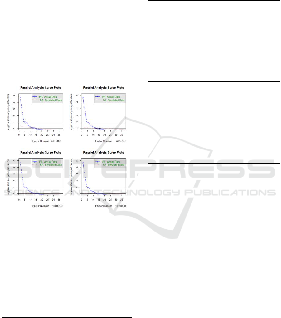
The right number of factors is determined by
parallel analysis. Figure 2 shows the number of
eigenvalues of the data that are greater than
simulated values. In other words, Parallel analysis
suggests that the numbers of factors are 11, 12, 12
and 12 for sample sizes 1000, 5000, 10000 and
20000 respectively.
Figure 2: Factor Numbers Using parallel analysis; Alarm
network.
As mentioned before, we sapmle 1000, 5000,
10000 and 20000 cases and repeat this procedure 10
times and report the mean of TPs, FPs, F-measures
and the standard deviation (std) of F-measures.
According to the Tables 1- 4, our proposed method
for determination of node ordering as input for K2
algorithm receives higher value of F-measure.
Table 1: Comparing different methods (Sample size: 1000,
network=Alarm).
Method TP FP F std
PROPOSED 22.12 44.37
0.39
0.011
K2 + MWST 16.25 44.38 0.3 0.031
K2-MWST 22.75 58.87 0.35 0.012
Chen et al. 20.62 58.62 0.32 0.023
Hruschka et al 20.87 61.50 0.32 0.019
Table 2: Comparing different methods (Sample size: 5000,
network =Alarm).
Method TP FP F std
PROPOSED 22.25 44.5
0.39
0.010
K2 + MWST 15.62 45.62 0.29 0.011
K2-MWST 22.25 57.12 0.35 0.022
Chen et al. 20.75 51.75 0.35 0.013
Hruschka et al 21.12 56.87 0.34 0.012
Table 3: Comparing different methods (Sample size:
10000, network =Alarm).
Method TP FP F std
PROPOSED 21.37 42.75
0.40
0.023
K2 + MWST 18.87 37.25 0.36 0.013
K2-MWST 18.25 46.50 0.33 0.012
Chen et al. 22.50 53.62 0.36 0.018
Hruschka et al 22.37 53.12 0.36 0.016
Table 4: Comparing different methods (Sample size:
20000, network =Alarm).
Method TP FP F
std
PROPOSED 22.37 36.12
0.41
0.020
K2 + MWST 16.50 45.50 0.30
0.021
K2-MWST 23.12 57.25 0.36
0.016
Chen et al. 23.12 52.37 0.38
0.014
Hruschka et
al
22.87 49.50 0.38
0.014
4.2 Hailfinder Network
Hailfinder is a BN designed to forecast severe
summer hail in northeastern Colorado. The number
of nodes and arcs are 56 and 66 respectively (Figure
3). The 56 nodes in Hailfinder network can be
viewed as ordinal variables; therefore the Spearman
correlation between variables can be considered for
performing FA.
Figure 4 shows the number of eigenvalues of the
data that are greater than simulated values. Parallel
analysis suggests that the numbers of factors are 13,
18, 19 and 21 for sample sizes 1000, 5000, 10000
and 20000 respectively.
A Simple Node Ordering Method for the K2 Algorithm based on the Factor Analysis
277
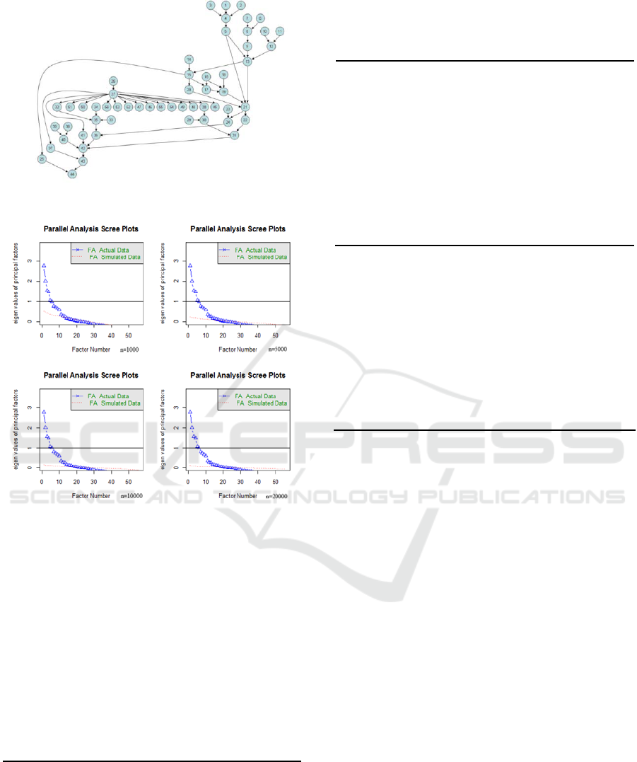
Figure 3: Hailfinder Network.
Figure 4: Factor Numbers Using parallel analysis;
Hailfinder.
We also sample 1000, 5000, 10000 and 20000
cases form Hailfinder and repeat this procedure 10
times and report the mean of TPs, FPs, F-measures
and the standard deviation of F-measures.
As shown in Tables 5-8, if we deal with a large
data set, our proposed method for determining the
node ordering among variables has higher accuracy
as input for K2 algorithm.
Table 5: Comparing different methods (Sample size: 1000,
network =Hailfinder).
Method TP FP F std
PROPOSED 29.37 72
0.35
0.013
K2 + MWST 20.5 64.5 0.27 0.012
K2-MWST 19.12 67.5 0.25 0.009
Chen et al. 20.87 60.62 0.28 0.011
Hruschka et al 26.37 81.12 0.3 0.010
Table 6: Comparing different methods Sample size: 5000,
network =Hailfinder).
Method TP FP F std
PROPOSED 28.12 63.25
0.35
0.015
K2 + MWST 21.87 61.62 0.29 0.012
K2-MWST 20.75 63.25 0.27 0.009
Chen et al. 22.87 61.62 0.30 0.012
Hruschka et al 25.12 73.25 0.30 0.014
Table 7: Comparing different methods (Sample size:
10000, network =Hailfinder).
Method TP FP F std
PROPOSED 31.12 62.12
0.39
0.013
K2 + MWST 22.00 61.87 0.29 0.015
K2-MWST 21.87 61.87 0.29 0.011
Chen et al. 26.25 58.75 0.34 0.011
Hruschka et al 25.75 62.37 0.33 0.017
Table 8: Comparing different methods (Sample size:
20000, network =Hailfinder).
Method TP FP F std
PROPOSED 33.12 58.5
0.42
0.017
K2 + MWST 27.75 61.75 0.35 0.019
K2-MWST 22.62 61.75 0.3 0.016
Chen et al. 22.75 61.87 0.3 0.010
Hruschka et al 31.00 65.87 0.38 0.013
5 COMPARISON OF CONSUMED
TIME AND COMPLEXITY
Yielding more effective node ordering is an
important issue for the K2 algorithm. However, the
most effective heuristic algorithm is the one
proposed by Chen et al. (2008) whose time is O(n
4
).
We introduce a very simple node ordering method as
input of K2 algorithm that the time complexity was
thereby reduced to O(n
2
). We also compare the time
consumption by the node ordering methods. In this
comparison, less time reflects better performance.
The results are presented in Table 9. It shows that
our method has the better performance. So we can
conclude that the proposed ordering method is much
accurate and simple compared with other ordering
space exploring approaches.
ICPRAM 2017 - 6th International Conference on Pattern Recognition Applications and Methods
278

Table 9: Time consumed (s) during node ordering
(including the K2 algorithm).
Method
Alarm Hailfinder
PROPOSED 8.98 s 31.35 s
K2 + MWST 11.28 s 33.62 s
K2-MWST 12.36 s 34.70 s
Chen et al. 75.19 s 300.94 s
Hrushka et al. 236.22 984.95 s
6 CONCLUSIONS
The BN-learning problem is NP-hard, so many
approaches have been proposed for this task is quite
complex and hard to implement. In this paper, we
propose a very simple and easy-to-implement
method for addressing this task. Our method is based
on the single order yielded by factor analysis. It does
not explore the space of the orderings. So, it is much
easier than ordering-based approaches which do
explore the ordering space. Because factor analysis
is based on the correlation matrix of the variables
involved.
REFERENCES
Abramson, B., Brown, J., Edwards, W., Murphy, A., &
Winkler, R. L. (1996). Hailfinder: A Bayesian system
for forecasting severe weather. International Journal
of Forecasting, 12(1), 57-71.
Beinlich, I. A., Suermondt, H. J., Chavez, R. M., &
Cooper, G. F. (1989).The ALARM monitoring system:
A case study with two probabilistic inference
techniques for belief networks (pp. 247-256). Springer
Berlin Heidelberg.
Chen, X. W., Anantha, G., & Lin, X. (2008). Improving
Bayesian network structure learning with mutual
information-based node ordering in the K2
algorithm. IEEE Transactions on Knowledge and Data
Engineering, 20(5), 628-640.
Chow, C., & Liu, C. (1968). Approximating discrete
probability distributions with dependence trees. IEEE
transactions on Information Theory, 14(3), 462-467.
Cooper, G. F., & Herskovits, E. (1992). A Bayesian
method for the induction of probabilistic networks
from data. Machine learning, 9(4), 309-347.
Friedman, N., & Goldszmidt, M. (1998). Learning
Bayesian networks with local structure. In Learning in
graphical models (pp. 421-459). Springer Netherlands.
Friedman, N., & Koller, D. (2000). Being Bayesian about
network structure. In Proceedings of the Sixteenth
conference on Uncertainty in artificial
intelligence (pp. 201-210). Morgan Kaufmann
Publishers Inc.
Geiger, D., Verma, T., & Pearl, J. (1990). Identifying
independence in Bayesian networks. Networks, 20(5),
507-534.
Ghahramani, Z. (1998). Learning dynamic Bayesian
networks. In Adaptive processing of sequences and
data structures (pp. 168-197). Springer Berlin
Heidelberg.
Grossman, D., & Domingos, P. (2004, July). Learning
Bayesian network classifiers by maximizing
conditional likelihood. In Proceedings of the twenty-
first international conference on Machine learning (p.
46). ACM.
Hayton, J. C., Allen, D. G., & Scarpello, V. (2004). Factor
retention decisions in exploratory factor analysis: A
tutorial on parallel analysis. Organizational research
methods, 7(2), 191-205.
Heckerman, D. (1998). A tutorial on learning with
Bayesian networks. In Learning in graphical
models (pp. 301-354). Springer Netherlands.
Hruschka, E. R., & Ebecken, N. F. (2007). Towards
efficient variables ordering for Bayesian networks
classifier. Data & Knowledge Engineering,63(2), 258-
269.
Horn, J. L. (1965). A rationale and test for the number of
factors in factor analysis. Psychometrika, 30(2), 179-
185.
Hsu, W. H., Guo, H., Perry, B. B., & Stilson, J. A. (2002,
July). A Permutation Genetic Algorithm For Variable
Ordering In Learning Bayesian Networks From Data.
In GECCO (Vol. 2, pp. 383-390).
Jensen, F. V. (1996). An introduction to Bayesian
networks (Vol. 210). London: UCL press.
Johnson, R. A., & Wichern, D. W. (2002). Applied
multivariate statistical analysis (Vol. 5, No. 8). Upper
Saddle River, NJ: Prentice hall.
Kaiser, Henry F. (1992). "On Cliff's formula, the Kaiser-
Guttman rule, and the number of factors." Perceptual
and motor skills 74.2: 595-598.
Kim, J. O., & Mueller, C. W. (1978). Factor analysis:
Statistical methods and practical issues (Vol. 14).
Sage.
Lamma, E., Riguzzi, F., & Storari, S. (2005). Improving
the K2 algorithm using association rule
parameters. Information Processing and Management
of Uncertainty in Knowledge-Based Systems
(IPMU04), 1667-1674.
Larranaga, P., Kuijpers, C. M., Murga, R. H., &
Yurramendi, Y. (1996). Learning Bayesian network
structures by searching for the best ordering with
genetic algorithms. IEEE transactions on systems,
man, and cybernetics-part A: systems and
humans, 26(4), 487-493.
Leray, P., & Francois, O. (2004). BNT structure learning
package: Documentation and
experiments. Laboratoire PSI, Universitè et INSA de
Rouen, Tech. Rep.
Madigan, D., York, J., & Allard, D. (1995). Bayesian
graphical models for discrete data. International
Statistical Review/Revue Internationale de Statistique,
215-232.
A Simple Node Ordering Method for the K2 Algorithm based on the Factor Analysis
279

Pearl, J. (1988). Probabilistic Reasoning in Intelligent
Systems. San Francisco, CA: Morgan Kaufmann.
Perrier, E., Imoto, S., & Miyano, S. (2008). Finding
optimal Bayesian network given a super-
structure. Journal of Machine Learning
Research,9(Oct), 2251-2286.
Powers, D. M. (2011). Evaluation: from precision, recall
and F-measure to ROC, informedness, markedness
and correlation, Journal of machine Learning
technologies, 2(1), 37-63.
Ruiz, C. (2005). Illustration of the K2 algorithm for
learning Bayes net structures. Department of
Computer Science, WPI.
Romero, T., Larrañaga, P., & Sierra, B. (2004). Learning
Bayesian networks in the space of orderings with
estimation of distribution algorithms. International
Journal of Pattern Recognition and Artificial
Intelligence, 18(04), 607-625.
Spirtes, P., Glymour, C., & Scheines, R. (2000).
Causation, Prediction, and Search. Adaptive
Computation and Machine Learning Series. The MIT
Press, 49, 77-78.
ICPRAM 2017 - 6th International Conference on Pattern Recognition Applications and Methods
280
