Adaptive Rendering based on Adaptive Order Selection

Hongliang Yuan

1,2

, Changwen Zheng

, Quan Zheng

1,2

and Yu Liu

1,2

Institute of Software, Chinese Academy of Sciences, Beijing, China

University of Chinese Academy of Sciences, Beijing, China

Keywords:

Adaptive Rendering, Adaptive Order Selection, Monte Carlo Ray Tracing, Mean Squared Error.

Abstract:

We propose a new adaptive sampling and reconstruction method based on a novel, adaptive order polynomial

ﬁtting which can preserve various high-frequency features in generated images and meanwhile mitigate the

noise efﬁciently. Some auxiliary features have strong linear correlation with luminance intensity in the smooth

regions of the image, but the relationship does not hold in the high-frequency regions. In order to handle

these cases robustly, we approximate luminance intensity in the auxiliary feature space by constructing local

polynomial functions with order varying adaptively. Firstly, we sample the image space uniformly. Then

we decide the order of ﬁtting with the least estimated mean squared error (MSE) for each pixel. Finally,

we distribute additional ray samples to areas with higher estimated MSE if sampling budget remains. We

demonstrate that our method makes signiﬁcant improvement in terms of both numerical error and visual quality

compared with the state-of-the-art.

1 INTRODUCTION

Monte Carlo (MC) ray tracing (Kajiya, 1986) is the

commonly acknowledged efﬁcient algorithm to syn-

thesize photo-realistic images from 3D models. How-

ever, the rendered images generated by MC ray trac-

ing at low sampling rate are noisy, and generating

noise-free images needs dozens of hours. In order to

synthesize satisfactory images in reasonable time, re-

moving MC noise in image-space has been actively

studied recently. The model of ﬁltering MC noise can

be formulated as:

y = m(x) +ε (1)

where y is a scalar response variable, x = (x

, ..., x

)

is a d-dimensional vector of explanatory variables and

ε represents MC noise.

From the perspective of rendering, m(x) and y de-

note an unknown ground truth image and a noisy im-

age, respectively. The vector x contains spatial and

range components of the image, as well as additional

geometric information including surface normal, tex-

ture color and direct illumination visibility and so on.

The additional geometric information, which is also

called the auxiliary features, is computed at every

pixel where we average out geometries collected from

multiple sample rays.

Image-space denoising locally approximates the

color value of a pixel c as a weighted average of its

neighbors:

ˆm(x

;H) =

∑

i∈Ω

(i, c)

∑

i∈Ω

(i, c)

(2)

where ˆm(x

;H) is the ﬁltered color value of pixel c, y

is the input color value of pixel i, Ω

is a local window

centered on c and K

(·) denotes a nonnegative weight

function with a bandwidth matrix H. The equation

is called Nadaraya-Watson (Nadaraya, 1964; Watson,

1964) estimator which is the weighted least square so-

lution of the following optimization problem:

min

∑

i∈Ω

− α)

(i, c) (3)

i.e., ˆm(x

;H) =

α. The solution can be also expressed

as follows:

α = e

WX)

−1

= L

(4)

where e = (1)

, Y = (y

, ..., y

)

and n represents

the number of pixels within a ﬁltering window cen-

tered on c, W = diag(K

(1, c), ..., K

(n, c)) and X =

(1, ..., 1)

. L

) is called equivalent kernel. The

bilateral ﬁlter (Tomasi and Manduchi, 1998) is an

example of Nadaraya-Watson estimator. The weight

(i, c) is deﬁned as:

(i, c) = exp



−ki − ck

2σ



exp



−ky

− y

2σ



(5)

Yuan H., Zheng C., Zheng Q. and Liu Y.

Adaptive Rendering based on Adaptive Order Selection.

DOI: 10.5220/0006093100370045

In Proceedings of the 12th International Joint Conference on Computer Vision, Imaging and Computer Graphics Theory and Applications (VISIGRAPP 2017), pages 37-45

ISBN: 978-989-758-224-0

so that the bandwidth matrix H =

diag(σ

, σ

). The non-local means

(NL-Means) ﬁlter (Buades et al., 2008) is also a

generalization of Nadaraya-Watson estimator where

the weight is computed based on small patches.

From the Equation 4, we know the Nadaraya-Watson

estimator

α is a locally weighted average of the

response variables in the neighborhood of the given

pixel c.

The Nadaraya-Watson estimator converges more

slowly at the boundary and its conditional variance

is larger in practice for points on the boundary than

for points on the interior. Moon et al. (Moon et al.,

2014) introduces a local linear estimator to remove

MC noise:

min

α,β

∑

i∈Ω

− α −β

− x

))

(i, c) (6)

Its solution is also expressed as the Equation 4, but

e = (1, 0, ..., 0)

is a (d + 1)-dimensional vector and

the ith row of X is set as (1, (x

− x

)

Intuitively it is clear that in the smooth region

of the image the Nadaraya-Watson estimator or lo-

cal linear estimator is preferable, whereas in the high-

frequency region due to MC effects such as motion

blur and depth-of-ﬁeld, polynomials of higher or-

der such as local cubic estimator is recommendable.

Hence, the order of local polynomial ﬁtting should be

varied to reﬂect the local curvature of the unknown

ground truth image.

Based on previous analysis, we present a novel,

adaptive order polynomial ﬁtting based adaptive sam-

pling and reconstruction method to effectively han-

dle various MC rendering effects (e.g., motion blur,

depth-of-ﬁeld, soft shadow, etc). Given a ﬁxed spatial

bandwidth, our method estimates an unknown func-

tion based on a data-driven variable order selection

procedure. Our core idea is to develop a robust esti-

mate of the MSE of each pixel and to use this estimate

as a criterion for adaptive order selection (AOS), i.e.

varying the order of the Taylor series approximation.

Our idea is based on obvious observations that a ref-

erence image in the area of motion blur no longer has

a linear correlation with given auxiliary features (e.g.,

textures). Speciﬁcally, we make the following techni-

cal contributions: For a given ﬁxed spatial bandwidth

and each order (i.e., local linear estimator and local

cubic estimator), our method estimates the MSE of

each pixel which is decomposed into estimation of

bias and variance terms. The local optimal order is

selected with the least MSE.

2 PREVIOUS WORK

Adaptive sampling and reconstruction was pioneered

by Kajiya (Kajiya, 1986). The key of adaptive sam-

pling is to develop a robust error metric which can

guide where we need to allocate more ray sam-

ples. Common error metrics includes Stein’s Unbi-

ased Risk Estimator (SURE) (Stein, 1981), contrast

metric (Mitchell, 1987), median absolute deviation

(MAD) (Donoho and Johnstone, 1994), MSE which

can be decomposed into variance plus the square of

bias and so on. We will review the most recent adap-

tive renderings based on previous analysis and clas-

sify them into Nadaraya-Watson estimator, local lin-

ear estimator and higher order estimator.

Nadaraya-Watson Estimator. Li et al. (Li et al.,

2012) leverage cross-bilateral ﬁlter to ﬁlter MC noise.

They compute the weight between two pixels similar

to the Equation 5 as well as considering auxiliary fea-

tures. Sen et al. (Sen and Darabi, 2012) also use cross-

bilateral ﬁlter, but utilizing mutual information to

measure the relation between feature differences and

ﬁlter weights. Rousselle et al. (Rousselle et al., 2013)

adopt SURE to estimate MSE of three cross-bilateral

ﬁlters with the same spatial support, but different their

other parameters. Moon et al. (Moon et al., 2013) use

a virtual ﬂash image as a stopping function to com-

pute the weight of a cross-bilateral ﬁlter. Rousselle et

al. (Rousselle et al., 2012) exploit NL-Means ﬁlter for

adaptive rendering, while Delbracio et al. (Delbracio

et al., 2014) propose a multi-scale NL-Means ﬁlter

for adaptive reconstruction. Kalantari et al. (Kalan-

tari et al., 2015) present a machine learning approach

to reduce MC noise. These methods are all the cases

of the Nadaraya-Watson estimator.

Local Linear Estimator. Moon et al. (Moon et al.,

2014) construct local linear estimator to estimate the

color value of each pixel. Moon et al. (Moon et al.,

2015) propose to approximate the color value of each

pixel in a prediction window with multiple, but sparse

local linear estimators. Bitterli et al. (Bitterli et al.,

2016) study existing approaches and present nonlin-

early weighted ﬁrst-order regression for denoising

MC noise, which is also the case of local linear es-

timator, but computing the weight based on small

patches.

High Order Estimator. Most recently, Moon et al.

(Moon et al., 2016) locally approximate an image

with polynomial functions and the optimal order of

each polynomial function is estimated so that multi-

stage reconstruction error can be minimized. How-

GRAPP 2017 - International Conference on Computer Graphics Theory and Applications

ever, they construct polynomial functions only con-

sidering pixel position (2D). In contrast, we construct

higher order regression functions considering all aux-

iliary features and present a bias estimation leveraging

Taylor expansion.

There are some adaptive renderings which do

not belong to these categories. For example,

multi-dimensional adaptive rendering proposed by

Hachisuka et al. (Hachisuka et al., 2008), and adaptive

wavelet rendering presented by Overbeck et al. (Over-

beck et al., 2009).

3 LOCAL POLYNOMIAL

FITTING

Local linear estimator can locally estimate image

functions efﬁciently when non-linearity in the 2D im-

age space becomes nearly linear in the auxiliary fea-

ture space. This is deﬁnitely true in smooth region

of a noisy image, but in rendering, some MC effects

such as glossy highlights and defocused areas can be

nonlinear as shown in Fig. 1. In such cases, we had

better select higher order of regression function to re-

duce bias due to the curvature of the signal being re-

constructed.

(a) Reference

0.6 0.9 1.2

0.3

0.6

0.9

Texture intensity×10

Reference intensity×10

(b) Intensity on texture

0.94 0.96 0.98

0.1

0.2

Depth

Reference intensity

0.5 1.5 2.5

0.5

1.5

2.5

Texture intensity×10

Reference intensity×10

(d) Intensity on texture

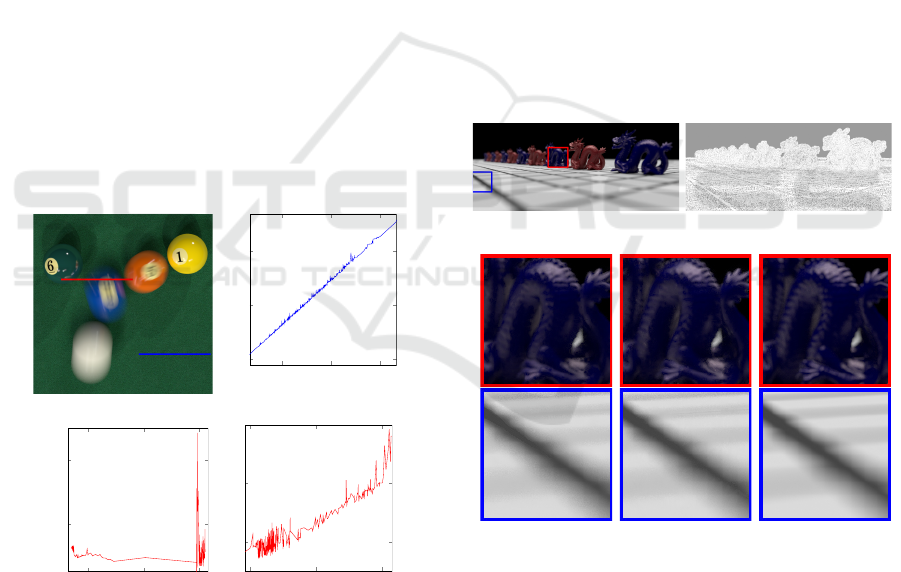
Figure 1: The reference image (a) is POOL scene gener-

ated with 32K ray samples per pixel. Intensity on texture

plot (b) is drawn from data in blue line of (a) which shows

strong linear correlation, where blue line is in smooth re-

gion. Intensity on depth plot (c) and on texture plot (d) are

drawn from data in red line of (a) respectively which shows

non-linearity, where red line covers smooth and motion blur

regions.

Based on our observations, we propose an adap-

tive order polynomial ﬁtting based method to recon-

struct smooth and high-frequency areas adaptively

and efﬁciently with ﬁxed spatial bandwidth. Bias will

increase and variance will decrease as bandwidth in-

creases. On the contrary, bias will decrease and vari-

ance will increase as bandwidth decreases. This is the

famous bias-variance trade-off issue. Bandwidth ro-

bustiﬁcation can be explained as follows. If the given

spatial bandwidth is too large, our method will choose

a higher order ﬁtting to reduce the bias. On the con-

trary, if the given spatial bandwidth is too small, our

method will select a lower order ﬁtting to reduce vari-

ance. As a result, this procedure adapts to smooth and

high-frequency regions of a MC input image.

Weighted local regression (WLR) proposed by

Moon et al. (Moon et al., 2014) uses local linear

estimator to approximate the nonlinear effects in a

high dimensional auxiliary feature space. It is sus-

ceptible to oversmooth the regions with high curva-

ture, even though they suggest a sophisticated two-

step optimization procedure. Fig. 2 demonstrates that

our method can improve the image quality compared

with WLR.

(a) OUR: 1500×636 (b) Adaptive order selection

rMSE 0.00045

(d) OUR 32 spp

rMSE 0.00037

(e) Reference

64K spp

Figure 2: Adaptive order selection image (b) is generated

when reconstructing our image (a), it is clear that in smooth

region (e.g., black region in (a)) local linear estimator indi-

cated by grey is optimal choice. Whereas, in high-frequency

regions (e.g., red and blue rectangle in (a)), local cubic esti-

mator indicated by white can preserve details efﬁciently, see

details comparison with WLR. Even though relative MSE

(rMSE deﬁned in Sec. 7) of WLR and our method is at

same order of magnitude, our method has an advantage over

WLR at the high-frequency regions from the perspective of

visual quality.

In order to perform AOS, we need ﬁt a high or-

Adaptive Rendering based on Adaptive Order Selection

der multivariate regression function. For the sake of

reducing computational overhead, we bring in partial

local polynomial regression. For example, we will use

the following design matrix for a local polynomial of

order v:

X =







1 (x

− x

)

. . . (x

− x

)

1 (x

− x

)

. . . (x

− x

)







(7)

where (x

−x

)

= ((x

−x

)

, ..., (x

−x

)

, i =

1, ..., n. The design matrix is only used for deciding

which order of ﬁtting can minimize the MSE at each

pixel. Once it is selected, we then estimate color value

and MSE which can guide the additional sampling.

Then, the optimization problem of higher order re-

gression can be written as follows:

min

∑

i=1

− β

−

∑

v=1

− x

)

− x

) (8)

where p is the order of the polynomial function,

β = (β

, β

, ..., β

)

, β

= (β

, ..., β

)

and (x

−

)

= ((x

− x

)

, ..., (x

− x

)

). K

(i, c) =

exp



−ki−ck



, since we only optimize the order of

local polynomial function, we select ﬁxed spatial ﬁl-

tering window h. Solving (8) by the least squares

method provides the solution:

β(x

) = (X

WX)

−1

WY (9)

whose conditional mean and variance are:

β(x

)|x

, ..., x

) = (X

WX)

−1

= (X

WX)

−1

W(Xβ + r)

= β + (X

WX)

−1

(10)

var(

β(x

)|x

, ..., x

) = (X

WX)

−1

×(X

WX)

−1

)

(11)

where m = (m(x

), ..., m(x

))

denotes the unknown

ground truth image and r = m − Xβ represents bias

image between the unknown ground truth image and

estimated image. Since r contains unknown term m,

we need to estimate it (Sec. 4).

4 ADAPTIVE ORDER

SELECTION

Fan et al. (Jianqing Fan, 1995a) proposed to use the

estimated MSE as a criterion to opt for the best or-

der of regression function, but their method can only

apply to regression function with one response vari-

able. Motivated by the previous work, we present

MSE estimation for multivariate regression. We in-

troduce bias estimation ﬁrst.

Bias Estimation. We estimate bias vector r = m −

Xβ = (r

, ..., r

)

via Taylor expansion

≈

p+a

∑

v=p+1

− x

)

≡ ξ

(12)

where a is an order which is greater than the approx-

imation order p. Fan et al. (Jianqing Fan, 1995b) dis-

cuss the choice of the approximation order, who sug-

gest to use a = 2 for practical implementation. In this

paper, we follow this recommendation. The unknown

bias in ξ = (ξ

, ..., ξ

)

can be estimated by ﬁtting

a local polynomial with the order p + a and the spa-

tial bandwidth h deﬁned previously. Let

∗

p+1

,...,

∗

p+a

be the locally weighted least squares estimation, then

∑

p+a

v=p+1

∗T

−x

)

. Bias at pixel c is estimated

bias

) = (X

WX)

−1

ξ (13)

Variance Estimation. After ﬁtting a local poly-

nomial with order p + a, the estimation result

ˆm(x

;H) can be expressed by

∑

i=1

, where

) is the item of row 0 and column i of matrix

∗T

∗

)

−1

∗T

W, then

∗2

) =

∑

i=1

))

) (14)

where X

∗

and W

∗

are the design matrix and weight

matrix respectively for the local (p + a)th order poly-

nomial ﬁtting. σ

) is the mean sample variance at

pixel i. Substituting (14) into (11) produces an ap-

proximated variance matrix:

var

) = (X

WX)

−1

×(X

WX)

−1

∗2

)

(15)

MSE Estimation. Equation (13) is a (d × p +1)×1

bias vector for β, the ﬁrst item is the estimated

bias of β

, denoted by

bias

[0]. Equation (15) is a

(d × p + 1) × (d × p + 1) covariance matrix for β,

var

)[0][0] is the estimated variance of β

. Hence,

the MSE of ˆm(x

) is estimated by

[

MSE

;H) =

var

)[0][0] + (

bias

)[0])

(16)

Algorithm of AOS. With the estimated MSE in

equation (16), algorithm 1 describes the procedure of

AOS-based MSE estimation, sampling map generat-

ing and color value estimation for each pixel.

GRAPP 2017 - International Conference on Computer Graphics Theory and Applications

Algorithm 1: AOS-based adaptive rendering.

Input:

Local polynomial ﬁtting of order p

max

= 3 and

order increment a = 2, Auxiliary feature vector

and intensity y

generated by renderer

Output:

Sampling density for next iteration or ﬁnal ﬁl-

tered image

1: for each pixel do

2: Dimension reduction by truncated singular

value decomposition (Moon et al., 2014);

3: Fit a local polynomial function of order p

max

4: for each order l ∈ {1, 3} do

5: Get coefﬁcients for a local polynomial ﬁt-

ting of order l + a from step 3;

6: Estimate

[

MSE

;H) by equation (16);

7: end for

8: Choose order l for this pixel with the least esti-

mated

[

MSE

;H);

9: For each channel, compute ˆm(x

;H) using lo-

cal polynomial ﬁtting with order l;

10: end for

11: if Sampling budget remains then

12: return a sampling density based on

∆rMSE(x

)(Sec. 5);

13: else

14: return ˆm(x

;H);

15: end if

5 ADAPTIVE SAMPLING

The state-of-the-art adaptive rendering methods ((Li

et al., 2012), (Rousselle et al., 2013) and (Moon et al.,

2014; Moon et al., 2015)) adopt a common iterative

approach to distribute additional ray samples to the

regions with higher estimated MSE. In this paper, we

implement that iterative model. To guide our adaptive

sampling, we uniformly distribute a small number of

ray samples (e.g., four ray samples per pixel) at the

ﬁrst iteration. Then we estimate

[

MSE(x;H) by our

AOS-based reconstruction method with ﬁxed spatial

bandwidth and predict an error reduction ∆MSE(x) =

[

MSE(x;H) × n(x)

−4

d+4

for each pixel, where the error

reduction factor n(x)

−4

d+4

is derived in (Moon et al.,

2014) and n(x) is the number of ray samples which

has been already allocated.

Rousselle et al. (Rousselle et al., 2011) suggest

relative MSE which is based on human visual percep-

tion that is more sensitive to darker areas. Since then,

most of adaptive rendering methods (e.g., (Li et al.,

2012), (Rousselle et al., 2012; Rousselle et al., 2013)

and (Moon et al., 2014; Moon et al., 2015)) adopt

that suggestion. The relative MSE is computed as fol-

lows: ∆rMSE(x) =

∆MSE(x)

ˆm

(x;H)+ε

, ε is a small number,

e.g., 0.0001, which is used to avoid a divide-by-zero.

If sampling budget still remains, we allocate ray sam-

ples per pixel which are proportional to ∆rMSE(x).

6 IMPLEMENTATION DETAIL

We implement our AOS-based adaptive rendering

method using CUDA on top of PBRT2 (Pharr and

Humphreys, 2010). The auxiliary features contain 10

dimensions: 2D pixel position, 1D depth, 3D texture,

3D normal and 1D direct illumination visibility. We

normalize auxiliary features to the range [0,1]. We

ﬁnd that the direct illumination visibility is very noisy

at low sampling rate, so we preﬁlter direct illumina-

tion visibility leveraging a non-local means ﬁlter in

an 10 × 10 window with patch size 6 × 6 as was done

in Rousselle et al. (Rousselle et al., 2013) and Kalan-

tari et al. (Kalantari et al., 2015). Even though other

features have less noise than visibility, we also apply

non-local means ﬁltering for them.

In order to continue to reduce the noise and mit-

igate the curse of dimensionality in multivariate re-

gression, we apply the truncated singular value de-

composition (Moon et al., 2014) to auxiliary features

within given ﬁltering window. In all our tests, we use

a 11×11 ﬁltering window in the iterative steps and

19×19 ﬁltering window in the ﬁnal step. The reason

why we use smaller ﬁltering windows in the iterative

stage is that we only estimate relative MSE. This de-

cision has only a slight effect on adaptive sampling.

We opt for a small number of iterations (i.e., 3) for

adaptive sampling.

We tested two orders of local polynomial ﬁtting,

one order is 1 which leads to local linear estimator and

the other is 3 which leads to local cubic estimator. All

the choice of the order of ﬁtting is odd-order, because

the asymptotic variance becomes large when moving

from an odd-order estimation to its consecutive even-

order estimation.

7 RESULTS AND DISCUSSIONS

We test our method using a mobile workstation

with Intel Core i7-4700MQ CPU @2.40GHz, and

NVIDIA Quadro K1100M with CUDA 7.5 SDK

for accelerating our proposed reconstruction method

based on adaptive order selection (AOS). We com-

pare our method with low discrepancy (Dobkin et al.,

Adaptive Rendering based on Adaptive Order Selection

1996) (LD) and the state-of-the-art adaptive render-

ing methods including WLR (Moon et al., 2014),

APR (Moon et al., 2016) and LBF (Kalantari et al.,

2015). To evaluate the WLR and LBF method, we use

the source code provided by authors and set param-

eters recommended by their corresponding papers.

Since the authors of APR method didn’t make their

source code public, we implemented their algorithm

on the CPU using the Eigen 3 library for efﬁcient

matrix operations. Even though our implementation

might not reach the same image quality as in their

original paper, it demonstrates that locally changing

polynomial function order can generate high-quality

image.

For purpose of comparing image quality gener-

ated by different methods in terms of a quantitative

measure, we introduce the relative mean squared er-

ror (rMSE) (Rousselle et al., 2011) which is deﬁned

as:

∑

i=1

( ˆm(x

)−m(x

))

m(x

)

+ε

, where ε = 0.001 prevents a

divide by zero, m(x) refers to the ground truth image.

We also use the structural similarity (SSIM) (Wang

et al., 2004) index to measure the similarity between

two images.

We evaluate our method on rendering following

scenes: POOL (1024×1024), SANMIGUEL (1024×

1024), SIBENIK (1024 × 1024) and TEAPOT

(1024 × 1024). These scenes include a variety of MC

effects, e.g., motion blur, depth-of-ﬁeld, soft shadow,

glossy reﬂection and so on. For each comparison,

we adopt equal-sample comparison with LBF and

WLR method, and equal-time comparison with LD

method. Our method and WLR implement adaptive

sampling, while LBF method only implement uni-

form sampling. Considering this case, all methods

adopt uniform sampling for SANMIGUEL scene.

Motion Blur Scene Comparison. The POOL

scene, in which three billiard balls have different mo-

tion directions, is used to compare motion blur effect

for different methods. Fig. 3 shows comparison re-

sults. LD generates noisy result even with larger ray

samples than other methods. LBF leaves artifacts in

the motion blur regions (blue box). The reason is

that LBF does not implement adaptive sampling and

rendering motion blur effect needs more ray samples.

APR method can preserve high-frequency edge while

WLR gives oversmoothed it (red box). Our method

not only generates a high-quality reconstruction re-

sult on the motion blurred regions but also preserves

soft shadows clearly. In addition, our method obtains

a lower rMSE and higher SSIM than other methods.

Complex Scene Comparison. The SANMIGUEL

scene has complex geometric structure with more

than 10 million triangles due to the use of object in-

stancing and is widely used for adaptive rendering

techniques. Fig. 4 illustrates comparison results. LD

method produces a very noisy image. Our method

preserves the edge and textures on wall (closeup in

red box) and the foliage details as well as the small di-

rect soft shadows (closeup in blue box). APR method

can preserve high-frequency edge and also the foliage

details. WLR fails to preserves edge and LBF tends

to blur textures on wall and the foliage details. Over-

all, our method generates more visual pleasing images

than other techniques.

Depth-of-ﬁeld Scene Comparison. Fig. 5 illus-

trates depth-of-ﬁeld effect comparison using the

SIBENIK scene, which has an environment light

which can be seen by refraction through the win-

dows. LBF and WLR produces an over-blurred fence

(closeup in blue box). Our method, on the other hand,

preserves the fence as on the reference image.

Glossy Reﬂection Scene Comparison. The

TEAPOT scene (Fig. 6) with glossy reﬂection and

high-frequency bump mapping on the ﬂoor is rec-

ognized as a challenging scene. LD produces noisy

image even with more than two times ray samples

than ours. All methods fail to reconstruct the bump

map (closeup in blue box) well. In addition, our

method preserves glossy highlights more accurately

than WLR which is inclined to oversmooth glossy

regions (closeup in red box).

Convergence Comparison. We also plot conver-

gence rate for the POOL and SANMIGUEL scenes

comparing with LD, LBF and WLR methods, see

Fig. 7. Our method and WLR adopt adaptive sam-

pling for the POOL scene. Considering that LBF

method does not implement adaptive sampling, all the

methods use uniform sampling for the SANMIGUEL

scene.

8 CONCLUSIONS

We have proposed a novel, adaptive order polyno-

mial ﬁtting based adaptive rendering approach for

efﬁciently denoising images with diverse MC ef-

fects. Given ﬁxed spatial bandwidth, we handle bias-

variance trade-off by varying order of polynomial ﬁt-

ting. For the given two choices of the order of ﬁt-

ting, we estimate the MSE for each pixel and select

GRAPP 2017 - International Conference on Computer Graphics Theory and Applications

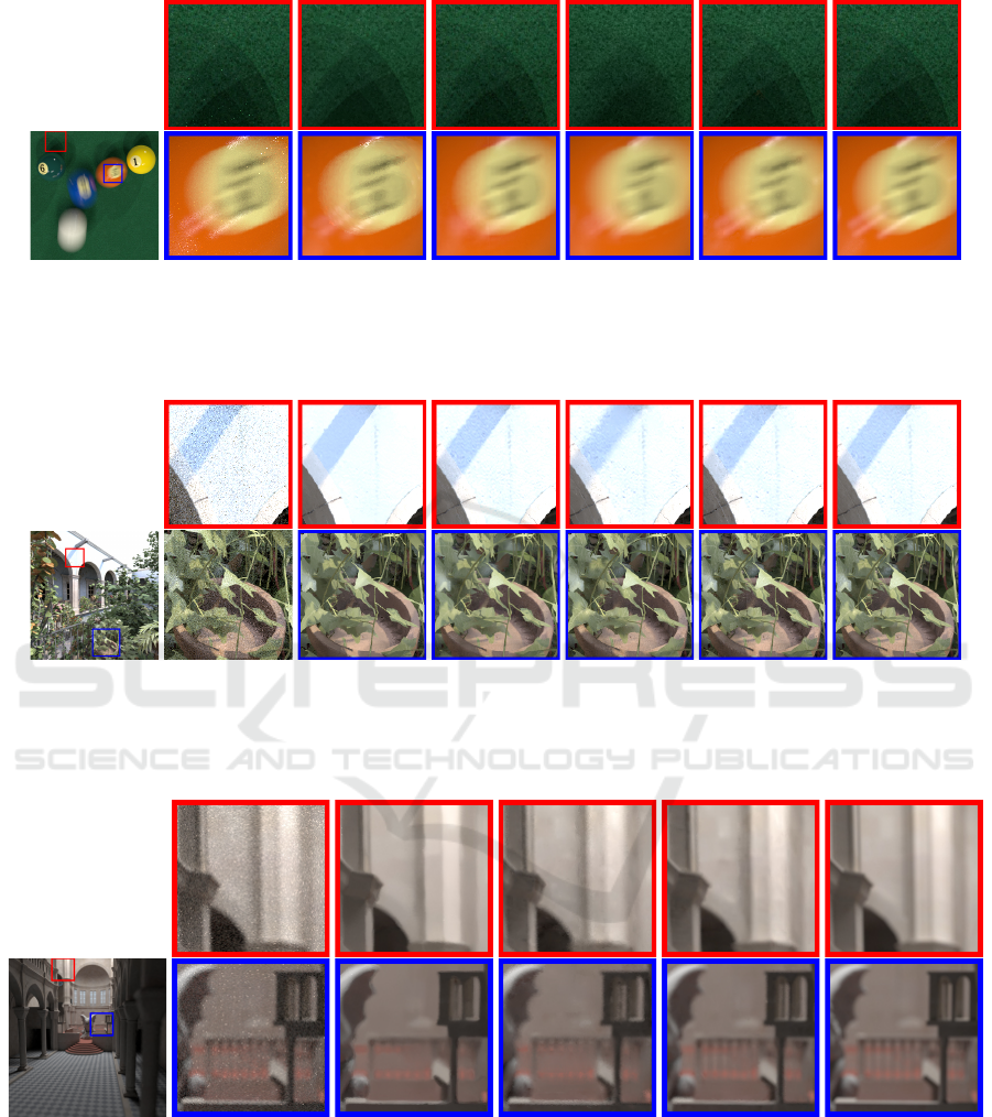
(a) OUR

rMSE:

SSIM:

(b) LD

118 spp (175 s)

0.00883

0.947

32 spp (169 s)

0.00109

0.959

(d) APR

32 spp (967 s)

0.00032

0.984

(e) WLR

32 spp (216 s)

0.00049

0.978

(f) OUR

32 spp (178 s)

0.00034

0.984

(g) Reference

64K spp

Figure 3: Motion blur scene comparison.

(a) OUR

rMSE:

SSIM:

(b) LD

196 spp (861 s)

0.03057

0.721

128 spp (892 s)

0.0102

0.879

(d) APR

128 spp (1883s)

0.0070

0.939

(e) WLR

128 spp (883 s)

0.0098

0.890

(f) OUR

128 spp (865 s)

0.0076

0.936

(g) Reference

64K spp

Figure 4: Complex scene comparison.

(a) OUR

rMSE:

SSIM:

(b) LD

56 spp (175 s)

0.01043

0.863

16 spp (163 s)

0.00083

0.960

(d) WLR

16 spp (185 s)

0.00106

0.947

(e) OUR

16 spp (171 s)

0.00067

0.973

(f) Reference

64K spp

Figure 5: Depth of ﬁeld scene comparison.

the order of ﬁtting with the least estimated MSE adap-

tively. We also distribute additional ray samples to the

regions with higher estimated MSE iteratively. We

compare our method with the state-of-the-art meth-

ods on a wide variety of MC distributed effects. The

comparison shows that our method enhances the im-

age quality in terms of both numerical error and visual

quality over the previous methods. In the future, we

Adaptive Rendering based on Adaptive Order Selection

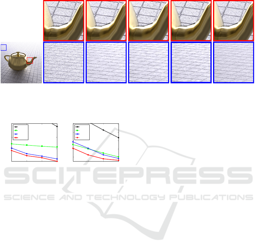
(a) OUR

rMSE:

SSIM:

(b) LD

156 spp (243 s)

0.0409

0.724

64 spp (246 s)

0.0388

0.761

(d) WLR

64 spp (289 s)

0.0391

0.760

(e) OUR

64 spp (247 s)

0.0313

0.778

(f) Reference

64K spp

Figure 6: Glossy reﬂections scene comparison.

16 32 64 128

0.19

0.76

2.64

11.6

Ray samples per pixel

rMSE×1e-3

LBF

W LR

OU R

(a) POOL

16 32 64 128

0.01

0.02

0.04

0.08

0.16

Ray samples per pixel

rMSE

LBF

W LR

OU R

(b) SANMIGUEL

Figure 7: Convergence plots in LD, LBF, WLR and our

method. Our method outperforms other three methods

across all the tested ray samples per pixel.

will explore extension of AOS-based adaptive render-

ing to handle animated images.

REFERENCES

Bitterli, B., Rousselle, F., Moon, B., Guiti

an, J. A. I., Adler,

D., Mitchell, K., Jarosz, W., and Nov

ak, J. (2016).

Nonlinearly weighted ﬁrst-order regression for de-

noising Monte Carlo renderings. Comput. Graph. Fo-

rum, 35(4):107–117.

Buades, A., Coll, B., and Morel, J.-M. (2008). Nonlocal

image and movie denoising. Int. J. Comput. Vision,

76(2):123–139.

Delbracio, M., Mus

e, P., Buades, A., Chauvier, J., Phelps,

N., and Morel, J.-M. (2014). Boosting Monte Carlo

rendering by ray histogram fusion. ACM Trans.

Graph., 33(1):8:1–8:15.

Dobkin, D. P., Eppstein, D., and Mitchell, D. P.

(1996). Computing the discrepancy with applica-

tions to supersampling patterns. ACM Trans. Graph.,

15(4):354–376.

Donoho, D. L. and Johnstone, I. M. (1994). Ideal spa-

tial adaptation by wavelet shrinkage. Biometrika,

81(3):425–455.

Hachisuka, T., Jarosz, W., Weistroffer, R. P., Dale, K.,

Humphreys, G., Zwicker, M., and Jensen, H. W.

(2008). Multidimensional adaptive sampling and re-

construction for ray tracing. In ACM SIGGRAPH

2008 Papers, SIGGRAPH ’08, pages 33:1–33:10,

New York. ACM.

Jianqing Fan, I. G. (1995a). Adaptive order polynomial

ﬁtting: Bandwidth robustiﬁcation and bias reduction.

Journal of Computational and Graphical Statistics,

4(3):213–227.

Jianqing Fan, I. G. (1995b). Data-driven bandwidth selec-

tion in local polynomial ﬁtting: Variable bandwidth

and spatial adaptation. Journal of the Royal Statistical

Society. Series B (Methodological), 57(2):371–394.

Kajiya, J. T. (1986). The rendering equation. In Pro-

ceedings of the 13th Annual Conference on Computer

Graphics and Interactive Techniques, SIGGRAPH

’86, pages 143–150, New York. ACM.

Kalantari, N. K., Bako, S., and Sen, P. (2015). A machine

learning approach for ﬁltering Monte Carlo noise.

ACM Trans. Graph., 34(4):122:1–122:12.

Li, T.-M., Wu, Y.-T., and Chuang, Y.-Y. (2012). SURE-

based optimization for adaptive sampling and recon-

struction. ACM Trans. Graph., 31(6):194:1–194:9.

Mitchell, D. P. (1987). Generating antialiased images at low

sampling densities. In Proceedings of the 14th An-

nual Conference on Computer Graphics and Interac-

tive Techniques, SIGGRAPH ’87, pages 65–72, New

York. ACM.

Moon, B., Carr, N., and Yoon, S.-E. (2014). Adaptive

rendering based on weighted local regression. ACM

Trans. Graph., 33(5):170:1–170:14.

Moon, B., Iglesias-Guitian, J. A., Yoon, S.-E., and Mitchell,

K. (2015). Adaptive rendering with linear predictions.

ACM Trans. Graph., 34(4):121:1–121:11.

Moon, B., Jun, J. Y., Lee, J., Kim, K., Hachisuka, T., and

Yoon, S. (2013). Robust image denoising using a vir-

tual ﬂash image for monte carlo ray tracing. Comput.

Graph. Forum, 32(1):139–151.

GRAPP 2017 - International Conference on Computer Graphics Theory and Applications

Moon, B., McDonagh, S., Mitchell, K., and Gross, M.

(2016). Adaptive polynomial rendering. ACM Trans.

Graph., 35(4):40:1–40:10.

Nadaraya, E. A. (1964). On estimating regression. Theory

of Probability & Its Applications, 9(1):141–142.

Overbeck, R. S., Donner, C., and Ramamoorthi, R. (2009).

Adaptive wavelet rendering. In ACM SIGGRAPH Asia

2009 Papers, SIGGRAPH Asia ’09, pages 140:1–

140:12, New York. ACM.

Pharr, M. and Humphreys, G. (2010). Physically Based

Rendering: From Theory to Implementation. Morgan

Kaufmann Publishers Inc., San Francisco.

Rousselle, F., Knaus, C., and Zwicker, M. (2011). Adaptive

sampling and reconstruction using greedy error mini-

mization. ACM Trans. Graph., 30(6):159:1–159:12.

Rousselle, F., Knaus, C., and Zwicker, M. (2012). Adaptive

rendering with non-local means ﬁltering. ACM Trans.

Graph., 31(6):195:1–195:11.

Rousselle, F., Manzi, M., and Zwicker, M. (2013). Robust

denoising using feature and color information. Com-

put. Graph. Forum, 32(7):121–130.

Sen, P. and Darabi, S. (2012). On ﬁltering the noise from the

random parameters in Monte Carlo rendering. ACM

Trans. Graph., 31(3):18:1–18:15.

Stein, C. M. (1981). Estimation of the mean of a multi-

variate normal distribution. The Annals of Statistics ,

9(6):1135–1151.

Tomasi, C. and Manduchi, R. (1998). Bilateral ﬁltering for

gray and color images. In Proceedings of the Sixth

International Conference on Computer Vision, ICCV

’98, pages 839–, Washington, DC, USA. IEEE Com-

puter Society.

Wang, Z., Bovik, A. C., Sheikh, H. R., and Simoncelli,

E. P. (2004). Image quality assessment: From error

visibility to structural similarity. Trans. Img. Proc.,

13(4):600–612.

Watson, G. S. (1964). Smooth regression analysis. Sankhy:

The Indian Journal of Statistics, Series A (1961-2002),

26(4):359–372.

Adaptive Rendering based on Adaptive Order Selection