
Optimized Linear Imputation
Yehezkel S. Resheff
1,2
and Daphna Weinshall
1
1
School of Computer Science and Engineering, The Hebrew University, Jerusalem, Israel
2
Edmond and Lily Safra Center for Brain Sciences, The Hebrew University, Jerusalem, Israel
{heziresheff, daphna}@cs.huji.ac.il
Keywords:
Imputation.
Abstract:
Often in real-world datasets, especially in high dimensional data, some feature values are missing. Since most
data analysis and statistical methods do not handle gracefully missing values, the first step in the analysis
requires the imputation of missing values. Indeed, there has been a long standing interest in methods for the
imputation of missing values as a pre-processing step. One recent and effective approach, the IRMI stepwise
regression imputation method, uses a linear regression model for each real-valued feature on the basis of all
other features in the dataset. However, the proposed iterative formulation lacks convergence guarantee. Here
we propose a closely related method, stated as a single optimization problem and a block coordinate-descent
solution which is guaranteed to converge to a local minimum. Experiments show results on both synthetic and
benchmark datasets, which are comparable to the results of the IRMI method whenever it converges. However,
while in the set of experiments described here IRMI often diverges, the performance of our methods is shown
to be markedly superior in comparison with other methods.
1 INTRODUCTION
Missing data imputation is an important part of data
preprocessing and cleansing (Horton and Kleinman,
2007; Pigott, 2001), since the vast majority of com-
monly applied supervised machine learning and sta-
tistical methods for classification rely on complete
data (Garc
´
ıa-Laencina et al., 2010). The most com-
mon option for many applications is to discard com-
plete records in which there are any missing values.
This approach is insufficient for several reasons: first,
when missing values are not missing at random (Lit-
tle, 1988; Heitjan and Basu, 1996), discarding these
records may bias the resulting analysis (Little and
Rubin, 2014). Other limitations include the loss of
information when discarding the entire record. Fur-
thermore, when dealing with datasets with either a
small number of records or a large number of features,
omitting complete records when any feature value is
missing may result in insufficient data for the required
analysis.
Early methods for data imputation include meth-
ods for replacing a missing value by the mean or me-
dian of the feature value across records (Engels and
Diehr, 2003; Donders et al., 2006). While these val-
ues may indeed provide a “good guess” when there is
no information present, this is often not case. Namely,
for each missing feature value there are other non-
missing values in the same record. It is likely there-
fore (or indeed, we assume) that other features contain
information regarding the missing feature, and impu-
tation should therefore take into account known fea-
ture values in the same record. This is done by subse-
quent methods.
Multiple imputation (see (Rubin, 1996) for a de-
tailed review) imputes several sets of missing values,
drawn from the posterior distribution of the missing
values under a given model, given the data. Subse-
quent processing is then to be performed on each ver-
sion of the imputed data, and the resulting multiple
sets of model parameters are combined to produce a
single result. While extremely useful in traditional
statistical analysis and public survey data, it may not
be feasible in a machine learning setting. First, the
run-time cost of performing the analysis on several
copies of the full-data may be prohibitive. Second,
being a model-based approach it depends heavily on
the type and nature of the data, and can’t be used as an
out-of-the-box pre-processing step. More importantly
though, while traditional model parameters may be
combined between versions of the imputed data (re-
gression coefficients for instance), many modern ma-
chine learning methods do not produce a representa-
tion that is straightforward to combine (consider the
Resheff, Y. and Weinshal, D.
Optimized Linear Imputation.
DOI: 10.5220/0006092900170025
In Proceedings of the 6th International Conference on Pattern Recognition Applications and Methods (ICPRAM 2017), pages 17-25
ISBN: 978-989-758-222-6
Copyright
c
2017 by SCITEPRESS – Science and Technology Publications, Lda. All rights reserved
17

parameters of an Artificial Neural Network or a Ran-
dom Forest for example
1
).
In (Raghunathan et al., 2001), a method for impu-
tation on the basis of a sequence of regression mod-
els is introduced. This method, popularized under the
acronym MICE (Buuren and Groothuis-Oudshoorn,
2011; Van Buuren and Oudshoorn, 1999), uses a non-
empty set of complete features which are known in
all the records as its base, and iteratively imputes one
feature at a time on the basis of the completed fea-
tures up to that point. Since each step produces a sin-
gle complete feature, the number of iterations needed
is exactly the number of features that have a missing
value in at least one record. The drawbacks of this
method are twofold. First, there must be at least one
complete feature to be used as the base. More im-
portantly though, the values imputed at the i −th step
can only use a regression model that includes the fea-
tures which were originally full or those imputed in
the i − 1 first steps. Ideally, the regression model for
each feature should be able to use all other feature
values.
The IRMI method (Templ et al., 2011) goes one
step further by building a sequence of regression mod-
els for each feature that can use all other feature val-
ues as needed. This iterative method initially uses a
simple imputation method such as median imputation.
In each iteration it computes for each feature the lin-
ear regression model based on all other feature values,
and then re-imputes the missing values based on these
regression models. The process is terminated upon
convergence or after a per-determined number of iter-
ations (Algorithm 1). The authors state that although
they do not have a proof of convergence, experiments
show fast convergence in most cases.
In Section 2 we present a novel method of Opti-
mized Linear Imputation (OLI). The OLI method is
related in spirit to IRMI in that it performs a linear
regression imputation for the missing values of each
feature, on the basis of all other features. Our method
is defined by a single optimization objective which we
then solve using a block coordinate-descent method.
Thus our method is guaranteed to converge, which is
its most important advantage over IRMI. We further
show that our algorithm may be easily extended to
use any form of regularized linear regression.
In Section 3 we ompare the OLI method to the
IRMI, MICE and Median Imputation (MI) methods.
1
In this case it would be perhaps more natural to train
the model using data pooled over the various copies of the
completed data rather than train separate models and aver-
age the resulting parameters and structure. This is indeed
done artificially in methods such as denoinsing neural nets
(Vincent et al., 2010), and has been known to be useful for
data imputation (Duan et al., 2014).
Using the same simulation studies as in the original
IRMI paper, we show that the results of OLI are rather
similar to the results of IRMI. With real datasets we
show that our method usually outperforms the alter-
natives MI and MICE in accuracy, while providing
comparable results to IRMI. However, IRMI did not
converge in many of these experimentsm while our
method always provided good results.
2 OLI METHOD
2.1 Notation
We start by listing the notation used throughout the
paper.
N Number of samples
d Number of features
x
i, j
The value of the j −th feature in the i−th
sample
m
i, j
Missing value indicators:
m
i, j
=
(
1 x
i, j
is missing
0 other wise
m
i
Indicator vector of missing values for for
the i −th feature
The following notation is used in the algorithms’
pseudo-code:
A[m] The rows of a matrix (or column vector)
A where the boolean mask vector m is
True
A[!m] The rows of a matrix (or column vector)
A where the boolean mask vector m is
False
linear
regression(X, y) A linear regression from the
columns of the matrix X to the target vec-
tor y, having the following fields:
.parameters: parameters of the fitted
model.
.predict(X): the target column y as pre-
dicted by the fitted model.
2.2 Optimization Problem
We formulate the linear imputation as a single opti-
mization problem. First we construct a design matrix:
X =
1
[x
i, j
(1 − m
i, j
)]
.
.
.
1
(1)
ICPRAM 2017 - 6th International Conference on Pattern Recognition Applications and Methods
18

Algorithm 1: The IRMI method for imputation of real-valued features (see (Templ et al., 2011) for more details).
input:
• X - data matrix of size N × (d + 1) containing N samples and d features
• m - missing data mask
• max iter - maximal number of iterations
output:
• Imputation values
1:
˜
X := median impute(X ) {assigns each missing value the median of its column}
2: while not converged and under max iter iterations do
3: for i := 1...d do
4: regression = linear regression(
˜
X
−i
[!m
i
],
˜
X
i
[!m
i
])
5:
˜
X
i
[m
i
] = regression.predict(
˜
X
−i
[m
i
])
6: end for
7: end while
8: return
˜
X − X
where the constant-1 rightmost column is used for the
intercept terms in the subsequent regression models.
Multiplying the data values x
i, j
by (1 − m
i, j
) simply
sets all missing values to zero, keeping non-missing
values as they are.
Our approach aims to find consistent missing
value imputations and regression coefficients as a sin-
gle optimization problem. By consistent we mean that
(a) the imputations are the values obtained by the re-
gression formulas, and (b) the regression coefficients
are the values that would be computed after the impu-
tations. We propose the following optimization for-
mulation:
min
A,M
||(X + M)A − (X + M)||
2
F
s.t. m
i, j
= 0 ⇒ M
i, j
= 0
M
i,d+1
= 0 ∀i
A
i,i
= 0 i = 1...d
A
i,d+1
= δ
i,d+1
∀i
(2)
where ||. ||
F
is the Frobenius norm.
Intuitively, the objective that we minimize mea-
sures the square error of reconstruction of the imputed
data (X +M), where each feature (column) is approx-
imated by a linear combination of all other features
plus a constant (that is, linear regression of the re-
maining imputed data). The imputation process by
which M is defined is guaranteed to leave the non-
missing values in X intact, by the first and second con-
straints which make sure that only missing entries in
X have a corresponding non-zero value in M. There-
fore:
(X + M) =
(
M f or missing values
X f or non missing values
The regression for each feature is further con-
strained to use only other features, by setting the di-
agonal values of A to zero (the third constraint). The
forth constraint makes sure that the constant-1 right-
most column of the design matrix is copied as-is and
therefore does not impact the objective.
We note that all the constraints set variables to
constant values, and therefore this can be seen as an
unconstrained optimization problem on the remaining
set of variables. This set includes the non-diagonal el-
ements of A and the elements of M corresponding to
missing values in X. We further note that this is not
a convex problem in A, M since it contains the MA
factor. In the next section we show a solution to this
problem that is guaranteed to converge to a local min-
imum.
2.3 Block Coordinate Descent Solution
We now develop a coordinate descent solution for the
proposed optimization problem. Coordinate descent
(and more specifically alternating least squares; see
for example (Hope and Shahaf, 2016)) algorithms are
extremely common in machine learning and statistics,
and while don’t guarantee convergence to a global op-
timum, they often preform well in practise.
As stated above, our problem is an unconstrained
optimization problem over the following set of vari-
ables:
{A
i, j
|i, j = 1, .., d; i 6= j} ∪ {M
i, j
|m
i, j
= 1}
Keeping this in mind, we use the following objective
function:
L(A, M) = ||(X + M)A − (X + M)||
2
F
(3)
=
d
∑
i=1
||(X + M)
−i
β
i
− (X + M)
i
||
2
F
(4)
Optimized Linear Imputation
19

Algorithm 2: Optimized Linear Imputation (OLI).
input:
• X
0
- data matrix of size N × d containing N samples and d features
• m- missing data mask
output:
• Imputation values
1: X := median impute(X
0
)
2: M := zeros(N, d)
3: A := zeros(d, d)
4: while not converged do
5: for i := 1...d do
6: β := linear regression(X
−i
, X
i
). parameters
7: A
i
:= [β
1
, ..., β
i−1
, 0, β
i
, ..., β
d
]
T
8: end for‘
9: while not converged do
10: M := M − α[(X + M)A − (X + M)](A − I)
T
11: M[!m] := 0
12: end while
13: X := X + M
14: end while
15: return M
where C
−i
denotes the matrix C without its i −th col-
umn, C
i
the i − th column, and β
i
the i − th column
of A without the i − th element (recall that the i − th
element of the i −th column of A is always zero). The
term (X + M)
−i
β
i
is therefore a linear combination
of all but the i − th column of the matrix (X + M).
The sum in (4) is over the first d columns only, since
the term added by the rightmost column is zero (see
fourth constraint in (2)).
We now suggest the following coordinate descent
algorithm for the minimization of the objective (3)
(the method is summarized in Algorithm 2):
1. Fill in missing values using median/mean (or any
other) imputation
2. Repeat until convergence:
(a) Minimize the objective (3) w.r.t. A (compute
the columns of the matrix A)
(b) Minimize the objective (3) w.r.t. M (compute
the missing values entries in matrix M)
3. Return M
2
As we will show shortly, step (a) in the iterative part
of the proposed algorithm reduces to calculating the
linear regression for each feature on the basis of all
other features, essentially the same as the first step in
the IRMI algorithm (Templ et al., 2011) Algorithm 1.
2
Alternatively, in order to stay close in spirit to the lin-
ear IRMI method, we may prefer to use (X + M)A as the
imputed data.
Step (b) can be solved either as a system of linear
equations or in itself as an iterative procedure, by gra-
dient descent on (3) w.r.t M using (5).
First, we show that step (a) reduces to linear re-
gression. Taking the derivatives of (4) w.r.t the non-
diagonal elements of column i of A we have:
∂L
∂β
i
= 2(X + M)
T
−i
[(X + M)
−i
β
i
− (X + M)
i
]
Setting the partial derivatives to zero gives:
(X + M)
T
−i
[(X + M)
−i
β
i
− (X + M)
i
]=0
⇒β
i
= ((X + M)
T
−i
(X + M)
−i
)
−1
(X + M)
T
−i
(X + M)
i
which is exactly the linear regression coefficients for
the i −th feature from all other (imputed) features, as
claimed.
Next, we obtain the derivatives of the objective func-
tion w.r.t M:
∇
M
=
∂L
∂M
= 2[(X + M)A − (X + M)](A − I)
T
(5)
leading to the following gradient descent algorithm
for step (b): step (b), Repeat until convergence:
(i) M := M − α∇
M
L(A, M)
(ii) ∀
i, j
: M
i, j
= M
i, j
m
i, j
where α is a predefined step size and the gradient is
given by (5). Step (ii) makes sure that only missing
ICPRAM 2017 - 6th International Conference on Pattern Recognition Applications and Methods
20

values are assigned imputation values
3
.
Our proposed algorithm uses a gradient descent
procedure for the minimization of the objective (3)
w.r.t M. Alternatively, one could use a closed form so-
lution by directly setting the partial derivative to zero.
More specifically, let
∂L
∂M
=0 (6)
Substituting (5) into (6), we get
M(A − I)(A − I)
T
= −X(A − I)(A − I)
T
which we rewrite as:
MP = Q (7)
with the appropriate matrices P, Q. Now, since only
elements of M corresponding to missing values of X
are optimization variables, only these elements must
be set to zero in the derivative (6), and hence only
these elements must obey the equality (7). Thus, we
have:
(MP)
i, j
= Q
i, j
∀i, j|m
i, j
= 1
which is a system of
∑
i, j
m
i, j
linear equations in
∑
i, j
m
i, j
variables.
2.4 Discussion
In order to better understand the difference between
the IRMI and OLI methods, we rewrite the IRMI it-
erative method (Templ et al., 2011) using the same
notation as used for our method. We start by defining
an error matrix:
E = (X + M)A − (X + M)
E is the error matrix of the linear regression models
on the basis of the imputed data. Unlike our method,
however, IRMI considers the error only in the non-
missing values of the data, leading to the following
objective function:
L(M, A) =
∑
i, j|m
i, j
=0
E
2
i, j
In order to minimize this loss function, at each
step the IRMI method (Algorithm 1) optimizes over a
single column of A (which in effect reduces to fitting
a single linear regression model), and then assigns as
3
Note that this is not a projection step. Recall that the
optimization problem is only over elements M
i j
where x
i j
is a missing value, encoded by m
i j
= 1. The element-wise
multiplication of M by m guarantees that all other elements
of M are assigned 0. Effectively, the gradient descent pro-
cedure does not treat them as independent variables, as re-
quired.
the missing values in the corresponding column of M
the values predicted for it by the regression model.
While this heuristic for choosing M is quite effective,
it is not a gradient descent step and it therefore leads
to a process with unknown convergence properties.
The main motivation for proposing our method was to
fix this shortcoming within the same general frame-
work and propose a method that is similar in spirit,
with a convergence guarantee.
Another advantage of the proposed formulation is
the ability to easily extend it to any regularized linear
regression. This can be done by re-writing the item-
ized form of the objective (4) as follows:
L(A, M) =
∑
i
[||(X + M)
−i
β
i
− (X + M)
i
||
2
F
+ Ω(β
i
)]
where Ω(β
i
) is the regularization term.
Now, assuming that the resulting regression prob-
lem can be solved (that is, minimizing each of the
summands in the new objective with a constant M),
and since step (b) of our method remains exactly the
same (the derivative w.r.t M does not change as the ex-
tra term does not depend on M), we can use the same
method to solve this problem as well.
Another possible extension is to use kernelized
linear regression. This may be useful in cases when
the dependencies between the features are not linear.
Here too we can use the same type of method of opti-
mization, but we defer to future research working out
the details of the derivative w.r.t M, which will obvi-
ously not remain the same.
The method of initialization is another issue de-
serving further investigation. Since our procedure
converges to a local minimum of the objective, it
may be advantageous to start the procedure from sev-
eral random initial points, and choose the best re-
sult. However, since the direct target (missing values)
are obviously unknown, we would need an alterna-
tive measure of the ”goodness” of a result. Since the
missing values are assumed to be missing at random,
it would make sense to use the distance between the
distributions of known and imputed values (per fea-
ture) as a measure of appropriateness of an imputa-
tion.
3 EXPERIMENTS
In order to evaluate our method, we compared its per-
formance to other imputation methods using various
types of data. We used complete datasets (real or syn-
thetic), and randomly eliminated entries in order to
simulate the missing data case. To evaluate the suc-
cess of each imputation method, we used the mean
Optimized Linear Imputation
21

square error (MSE) of the imputed values as a mea-
sure of error. MSE is computed as the mean square
distance between stored values (the correct values for
the simulated missing values) and the imputed ones.
In Section 3.1 we repeat the experimental evalua-
tion from (Templ et al., 2011) using synthetic data, in
order to compare the results of our method to the re-
sults of IRMI. In Section 3.2 we compare our method
to 3 other methods - IRMI, MI and MICE - using
standard benchmark datasets from the UCI repository
(Lichman, 2013) . In Section 3.3 we augment the
comparisons with an addition new reallife dataset of
storks migration data.
For some real datasets in the experiments de-
scribed below we report that the IRMI method did
not converge (and therefore did not return any re-
sult). This decision was reached when the MSE of
the IRMI method rose at least 6 orders of magnitude
throughout the allocated 50 iterations, or (when tested
with unlimited iterations) when it rose above the max-
imum valid number in the system of approximately
1e + 308.
3.1 Synthetic Data
The following simulation studies follow (Templ et al.,
2011) and compare OLI to IRMI. All simulations are
repeated 20 times with 10, 000 samples. 5% of all val-
ues across records are selected at random and marked
as missing. Values are stored for comparison with im-
puted values. Simulation data is multivariate normal
with mean of 1 in all dimensions. Unless stated oth-
erwise, the covariance matrix has 1 in its diagonal en-
tries and 0.7 in the off-diagonal entries.
The aim of the first experiment is to test the re-
lationship between the actual values imputed by the
IRMI and OLI methods. The simulation is based on
multivariate normal data with 5 dimensions. Results
show that the values imputed by the two methods are
highly correlated (Fig. 1a). Furthermore, the signed
error (original − imputed) is also highly correlated
(Fig. 1b). Together, these findings point to the sim-
ilarity in the results these two methods produce.
In the next simulation we test the performance of
the two methods as we vary the number of features.
The simulation is based on multivariate normal data
with 3 − 20 dimensions. The results (Fig. 2b) show
almost identical behavior of the IRMI and OLI al-
gorithms, which also coincides with the results pre-
sented for IRMI in (Templ et al., 2011). Median im-
putation (MI) is also shown for comparison as base-
line. Fig 3 shows a zoom into a small segment of
figure 2.
As expected, imputing the median (which is also
the mean) of each feature for all missing values re-
sults in an MSE equal to the standard deviation of the
features (i.e., 1). While very close, the IRMI and the
OLI methods do not return the exact same imputation
values and errors, with an average absolute deviation
of 0.053
Next we test the performance of the two methods
as we vary the covariance between the features. The
simulation is based on multivariate normal data with 5
dimensions. Non-diagonal elements of the covariance
matrix are set to values in the range 0.1 − 0.9. The re-
sults (Fig. 2a) show again almost identical behavior
of the IRMI and OLI algorithms. As expected, when
the dependency between the feature columns is in-
creased, which is measure by the covariance between
the columns (X-axis in Fig. 2a), the performance of
the regression-based methods IRMI and OLI is mono-
tonically improving, while the performance of the MI
method remain unaltered.
3.2 UCI Datasets
The UCI machine learning repository (Lichman,
2013) contains several popular benchmark datasets,
some of which have been previously used to compare
methods of data imputation (Schmitt et al., 2015).
In the current experiment we used the following
datasets: iris (Fisher, 1936), wine (white) (Cortez
et al., 2009), Ecoli (Horton and Nakai, 1996), Boston
housing (Harrison and Rubinfeld, 1978), and power
(T
¨
ufekci, 2014). Each feature of each dataset was
normalized to have mean 0 and standard deviation
of 1, in order to make error values comparable be-
tween datasets. Categorical features were dropped.
For each dataset, 5% of the values were chosen at
random and replaced with a missing value indica-
tor. The procedure was repeated 10 times. For these
datasets we also consider the MICE method (Buuren
and Groothuis-Oudshoorn, 2011) using the winMice
(Jacobusse, 2005) software.
The results are quite good, demonstrating the su-
perior ability of the linear methods to impute miss-
ing data in these datasets (Table 1, rows 1-5). In the
Iris dataset our OLI method achieved an average error
identical to IRMI, which successfully converged only
9 out of the 10 runs. Both outperformed the MI and
MICE standard methods. In the Ecoli dataset both
the IRMI and OLI methods performed worse than the
alternative methods, with MICE achieving the low-
est MSE. In the Wine dataset the IRMI failed to con-
verge in all 10 repetitions, while the OLI method out-
performed the MI and MICE methods. The IRMI
method outperformed all other methods in the Hous-
ing dataset, but failed to converge 7 out of 10 times
ICPRAM 2017 - 6th International Conference on Pattern Recognition Applications and Methods
22
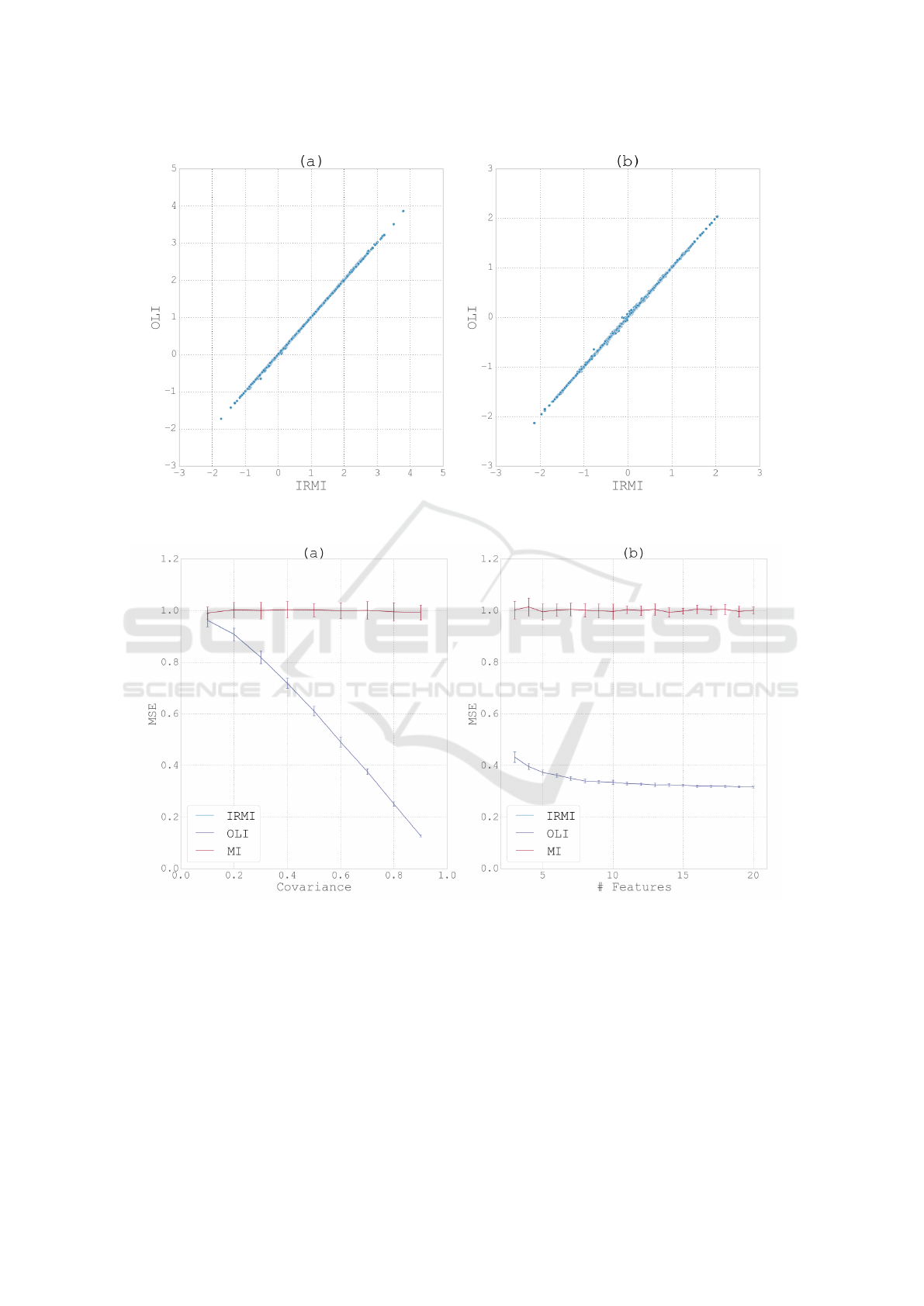
Figure 1: (a) Correlation between predicted values for missing data using the IRMI and OLI methods. (b) Correlation between
the signed error of the prediction for the two methods.
Figure 2: (a) MSE of the IRMI, OLI and MI methods as a function of the covariance. Data is 5 dimensional multivariate
normal. (b) MSE of the IRMI, OLI and MI methods as a function of the dimensionality, with a constant covariance of 0.7
between pairs of features. In both cases error bars represent standard deviation over 20 repetitions.
for the Power dataset.
In summary, in cases where the linear methods
were appropriate, with sufficient correlation between
the different features (shown in the second column
of Table 1), the proposed OLI method was com-
parable to the IRMI method with regard to mean
square error of the imputed values when the latter
converged, and superior in that it always converges
and therefore always returns a result. While the IRMI
method achieved slightly better results than OLI in
some cases, its failure to converge in others gives the
OLI method the edge. Overall, better results were
achieved for datasets with high mean correlation be-
tween features, as expected when using methods uti-
lizing the linear relationships between features.
Optimized Linear Imputation
23

Table 1: Comparison of the imputation results of the IRMI, OLI, MICE and MI methods with 5% missing data. The converged
column indicates the number of runs in which the IRMI method converged during testing; the MSE of IRMI was calculated
for converged repetitions only.
Dataset # Features correlation IRMI OLI MI MICE
converged MSE
Iris 4 0.59 9/10 0.20 0.20 1.00 0.33
Ecoli 7 0.18 9/10 8.26 5.75 1.72 1.20
Wine 11 0.18 0/10 - 0.87 1.05 1.10
Housing 11 0.45 10/10 0.28 0.30 1.14 0.56
Power 4 0.45 3/10 0.44 0.47 1.02 0.88
Storks 20 0.24 0/10 - 0.31 1.07 0.42
Figure 3: Zoom into a small part of figure 2.
3.3 Storks Behavioral Modes Dataset
In the field of Movement Ecology, readings from
accelerometers placed on migrating birds are used
for both supervised (Resheff et al., 2014) and unsu-
pervised (Resheff et al., 2015)(Resheff et al., 2016)
learning of behavioral modes. In the following ex-
periment we used a dataset of features extracted from
3815 such measurements. As with the UCI datasets,
10 repetitions were performed, each with 5% of the
values randomly selected and marked as missing. Re-
sults (Table 1, final row) of this experiment highlight
the relative advantage of the OLI method. While
the IRMI method failed to converge in all 10 repe-
titions, OLI achieved an average MSE considerably
lower than the MI baseline, and also outperformed the
MICE method.
4 CONCLUSION
Since the problem of missing values often haunts
real-word datasets while most data analysis methods
are not designed to deal with this problem, imputa-
tion is a necessary pre-processing step whenever dis-
carding entire records is not a viable option. Here
we proposed an optimization-based linear imputation
method that augments the IRMI (Templ et al., 2011)
method with the property of guaranteed convergence,
while staying close in spirit to the original method.
Since our method converges to a local optimum of a
different objective function, the two methods should
not be expected to converge to the same value ex-
actly. However, simulation results show that the re-
sults of the proposed method are generally similar
(nearly identical) to IRMI when the latter does indeed
converge.
The contribution of our paper is twofold. First,
we suggest an optimization problem based method for
linear imputation and an algorithm that is guaranteed
to converge. Second, we show how this method can
be extended to use any number of methods of regu-
larized linear regression. Unlike matrix completion
methods (Wagner and Zuk, 2015), we do not have
a low rank assumption. Thus, OLI should be pre-
ferred when data is expected to have some linear re-
lationships between features and when IRMI fails to
converge, or alternatively, when a guarantee of con-
vergence is important (for instance in automated pro-
cesses). We leave to future research the kernel exten-
sion of the OLI method.
REFERENCES
Buuren, S. and Groothuis-Oudshoorn, K. (2011). mice:
Multivariate imputation by chained equations in r.
Journal of statistical software, 45(3).
Cortez, P., Cerdeira, A., Almeida, F., Matos, T., and Reis,
J. (2009). Modeling wine preferences by data mining
from physicochemical properties. Decision Support
Systems, 47(4):547–553.
Donders, A. R. T., van der Heijden, G. J., Stijnen, T., and
Moons, K. G. (2006). Review: a gentle introduction
to imputation of missing values. Journal of clinical
epidemiology, 59(10):1087–1091.
Duan, Y., Yisheng, L., Kang, W., and Zhao, Y. (2014). A
ICPRAM 2017 - 6th International Conference on Pattern Recognition Applications and Methods
24

deep learning based approach for traffic data impu-
tation. In Intelligent Transportation Systems (ITSC),
2014 IEEE 17th International Conference on, pages
912–917. IEEE.
Engels, J. M. and Diehr, P. (2003). Imputation of missing
longitudinal data: a comparison of methods. Journal
of clinical epidemiology, 56(10):968–976.
Fisher, R. A. (1936). The use of multiple measurements in
taxonomic problems. Annals of eugenics, 7(2):179–
188.
Garc
´
ıa-Laencina, P. J., Sancho-G
´
omez, J.-L., and Figueiras-
Vidal, A. R. (2010). Pattern classification with miss-
ing data: a review. Neural Computing and Applica-
tions, 19(2):263–282.
Harrison, D. and Rubinfeld, D. L. (1978). Hedonic housing
prices and the demand for clean air. Journal of envi-
ronmental economics and management, 5(1):81–102.
Heitjan, D. F. and Basu, S. (1996). Distinguishing missing
at random and missing completely at random. The
American Statistician, 50(3):207–213.
Hope, T. and Shahaf, D. (2016). Ballpark learning: Estimat-
ing labels from rough group comparisons. Joint Eu-
ropean Conference on Machine Learning and Knowl-
edge Discovery in Databases, pages 299–314.
Horton, N. J. and Kleinman, K. P. (2007). Much ado about
nothing. The American Statistician, 61(1).
Horton, P. and Nakai, K. (1996). A probabilistic classifi-
cation system for predicting the cellular localization
sites of proteins. In Ismb, volume 4, pages 109–115.
Jacobusse, G. (2005). Winmice users manual. TNO Quality
of Life, Leiden. URL http://www. multiple-imputation.
com.
Lichman, M. (2013). UCI machine learning repository.
Little, R. J. (1988). A test of missing completely at random
for multivariate data with missing values. Journal of
the American Statistical Association, 83(404):1198–
1202.
Little, R. J. and Rubin, D. B. (2014). Statistical analysis
with missing data. John Wiley & Sons.
Pigott, T. D. (2001). A review of methods for missing data.
Educational research and evaluation, 7(4):353–383.
Raghunathan, T. E., Lepkowski, J. M., Van Hoewyk, J., and
Solenberger, P. (2001). A multivariate technique for
multiply imputing missing values using a sequence of
regression models. Survey methodology, 27(1):85–96.
Resheff, Y. S., Rotics, S., Harel, R., Spiegel, O., and
Nathan, R. (2014). Accelerater: a web application for
supervised learning of behavioral modes from accel-
eration measurements. Movement ecology, 2(1):25.
Resheff, Y. S., Rotics, S., Nathan, R., and Weinshall, D.
(2015). Matrix factorization approach to behavioral
mode analysis from acceleration data. In Data Science
and Advanced Analytics (DSAA), 2015. 36678 2015.
IEEE International Conference on, pages 1–6. IEEE.
Resheff, Y. S., Rotics, S., Nathan, R., and Weinshall, D.
(2016). Topic modeling of behavioral modes using
sensor data. International Journal of Data Science
and Analytics, 1(1):51–60.
Rubin, D. B. (1996). Multiple imputation after 18+
years. Journal of the American statistical Association,
91(434):473–489.
Schmitt, P., Mandel, J., and Guedj, M. (2015). A compari-
son of six methods for missing data imputation. Jour-
nal of Biometrics & Biostatistics, 2015.
Templ, M., Kowarik, A., and Filzmoser, P. (2011). Iterative
stepwise regression imputation using standard and ro-
bust methods. Computational Statistics & Data Anal-
ysis, 55(10):2793–2806.
T
¨
ufekci, P. (2014). Prediction of full load electrical power
output of a base load operated combined cycle power
plant using machine learning methods. Interna-
tional Journal of Electrical Power & Energy Systems,
60:126–140.
Van Buuren, S. and Oudshoorn, K. (1999). Flexible multi-
variate imputation by mice. Leiden, The Netherlands:
TNO Prevention Center.
Vincent, P., Larochelle, H., Lajoie, I., Bengio, Y., and
Manzagol, P.-A. (2010). Stacked denoising autoen-
coders: Learning useful representations in a deep net-
work with a local denoising criterion. The Journal of
Machine Learning Research, 11:3371–3408.
Wagner, A. and Zuk, O. (2015). Low-rank matrix recov-
ery from row-and-column affine measurements. arXiv
preprint arXiv:1505.06292.
Optimized Linear Imputation
25
