A Hierarchical Magniﬁcation Approach for Enhancing the Insight in

Data Visualizations

Stavros Papadopoulos, Anastasios Drosou and Dimitrios Tzovaras

Information Technologies Institute, Centre for Research and Technology Hellas, Thessaloniki, Greece

Keywords:

Data Visualization, Hierarchical, Magniﬁcation.

Abstract:

Non-linear deformations are useful for applications where users face highly cluttered visual displays, either

due to large datasets, or visualizations on small screens, or a combination of both, that increases the density

of the data and makes the perception of patterns difﬁcult. Non-linear deformations have been used to magnify

signiﬁcant/cluttered regions in data visualization, for the purpose of reducing clutter and enhancing the per-

ception of patterns. General deformation methods (e.g. logarithmic scaling and ﬁsh-eye views) suffer from

several drawbacks, since they do not consider the prominent features that must be preserved in the visualiza-

tion. This work introduces a hierarchical approach for non-linear deformation that aims to reduce visual clutter

by magnifying signiﬁcant regions, and lead to enhanced visualizations of two/three-dimensional datasets on

highly cluttered displays. The proposed approach utilizes an energy function, which aims to determine the

optimal deformation for every local region in the data, taking the information from multiple single-layer sig-

niﬁcance maps into account. The problem is subsequently transformed into an optimization problem for the

minimization of the energy function under speciﬁc spatial constraints. The proposed hierarchical approach

for the generation of the signiﬁcance map, surpasses current methods, and manages to efﬁciently identify

signiﬁcant regions and achieve better results.

1 INTRODUCTION

According to Rosenholtz et al.(Rosenholtz et al.,

2005) clutter is deﬁned as the state at which excess

items, or their representation or organization, leads to

a degradation of performance at some task. Visual

clutter(Ellis and Dix, 2007) can mislead users into de-

riving wrong conclusions, and increase the decision

conﬁdence on erroneous decisions. It can be caused

when large data volumes are visualized on small dis-

play devices, which reduce the visualization space

and its information capacity.

Non-linear deformations have been used to mag-

nify highly cluttered regions, and thus, reduce the

total cluttering in visualizations (Ellis and Dix,

2007)(Wu et al., 2013)(Tao et al., 2014). The

most commonly used functions for non-linear trans-

formations and clutter reduction are the logarithmic

and square root mappings(Maciejewski et al., 2013),

which do not take into account the content of the vi-

sualizations. According to Ellis et al. (Ellis and Dix,

2007), other popular methods for clutter reduction in-

clude: sampling/ﬁltering, changing the opacity of the

visual objects, and dimensional reordering. This work

focuses, only on non-linear transformations for clutter

reduction, since they can be used to create a general

approach that can be applied on multiple types of data

visualizations.

Towards reducing visual clutter on the visualiza-

tions, this work proposes a hierarchical magniﬁcation

approach for non-linear deformation. Building upon

the current state-of-the art, the proposed method en-

hances signiﬁcant regions of the data based on an un-

derling signiﬁcance map. It can be considered as a

focus+context technique, in which the focus points

are calculated automatically, based on their underly-

ing signiﬁcance. The proposed approach distributes

the distortion of the input data to regions of low sig-

niﬁcance, while signiﬁcant neighboring regions are

uniformly magniﬁed. In other words, although the de-

formation of all the cells in the grid is non-uniform,

small neighborhoods of signiﬁcant regions that have

similar signiﬁcance values, are magniﬁed by a simi-

lar amount, i.e. uniformly. This procedure results in

a deformation of the visualizations that reduces the

visual clutter, and enhances the analytics potential of

the visualizations.

The rest of this paper is organized as follows: Sec-

Papadopoulos S., Drosou A. and Tzovaras D.

A Hierarchical Magniﬁcation Approach for Enhancing the Insight in Data Visualizations.

DOI: 10.5220/0006073400290039

In Proceedings of the 12th International Joint Conference on Computer Vision, Imaging and Computer Graphics Theory and Applications (VISIGRAPP 2017), pages 29-39

ISBN: 978-989-758-228-8

tion 2 presents the related work on visualization de-

formation. The proposed magniﬁcation approach is

presented in Section 3. Section 4 illustrates the appli-

cation of the Magniﬁcation approach onto different

types of visualizations, as well as its comparison with

existing approaches. Finally, the paper concludes in

Section 5.

2 RELATED WORK

Over the last decade, many researchers have focused

their efforts on reducing visual clutter(Ellis and Dix,

2007) and capturing important properties of the data,

for extracting meaningful information. In this di-

rection several techniques dealing with clutter have

been proposed, like non-linear deformation, adjust-

ment of sampling ratios (Bertini and Santucci, 2006),

etc. Still, spatial deformation has been identiﬁed as

one of the most popular antagonists for clutter reduc-

tion (Ellis and Dix, 2007). Thereby, the positions of

the visual objects (e.g. a node of a graph, or a word

in context preserving word clouds) are displaced on

the display, so as to accommodate for the better visu-

alization of data patterns.

Regarding spatial deformation of the position/size

of the visual objects, Keim et al. (Keim et al., 2010)

presented the generalized scatterplots, a method to de-

form the positions of the points on the scatterplots and

reduce visual clutter. The authors also made use of

point displacement around the initial point of refer-

ence, in order to further reduce visual clutter in high

density areas. In the ﬁeld of ﬂow visualization, Tao et

al. (Tao et al., 2014) proposed the utilization of a 3D

deformation method, based on an entropy signiﬁcance

map. The proposed approach magniﬁes regions with

high entropy in the ﬂow visualizations, and reduces

visual clutter. Similarly, Wang et al. (Wang et al.,

2011) proposed a method for Focus+Context visual-

ization of volumetric data based on 3D grid deforma-

tion. The authors utilized a signiﬁcance map in or-

der to magnify important regions at the expense of re-

ducing the size of less signiﬁcant regions. The previ-

ous methods were only adjusted for speciﬁc visualiza-

tions, and they did not take the human perception for

clutter reduction into consideration. Based on these

limitations, Wu et al. (Wu et al., 2013) presented a

general visualization resizing framework, in order to

scale every visualization approach on small displays.

The authors utilized a clutter and a degree of interest

map in order to generate a 2-dimensional signiﬁcance

map. The positions of the data objects (i.e. scatterplot

point positions, graph layout, and word positions on a

context preserving word cloud) are distorted in order

to allow for the visualization of signiﬁcant visualiza-

tion areas on small screen sizes. The limitations of

the aforementioned approaches, are that they utilize

signiﬁcance maps created taking only one grid layer

with a speciﬁc resolution into account, and thus, they

lose important information. The introduction of the

hierarchical signiﬁcance map in this work is able to

more efﬁciently identify signiﬁcant regions, and pro-

vides better results.

The aforementioned methods deal only with

the spatial visual variables, which refer to the

size/position/shape of the visual objects. Very few

approaches have been proposed for non-spatial visual

variables, such as the color. For example, Thompson

et al. (Thompson et al., 2013) proposed a method for

color mapping that takes the input data distribution

into account. The authors produced palettes utiliz-

ing perceptual color distance, in order to emphasize

prominent values in the data. They also introduced

two different color mappings, one for the visual detec-

tion of large differences in data values, and one for the

visual detection of similar values, so that small differ-

ences can be detected. Eisemann et al. (Eisemann

et al., 2011) proposed the use of a simple projection

technique based on angular interpolation, in order to

distort the dataset before mapping its values to col-

ors. The user of the visualization can select the de-

sired distortion factor. Maciejewski et al. (Maciejew-

ski et al., 2013) utilized Box-Cox transformations for

transforming the distribution data, as close to a nor-

mal distribution as possible, before applying a color

scheme for choropleth maps. Unlike previous meth-

ods, the approach proposed in this paper is applied on

both spatial and non-spatial visual variables.

Towards the direction of reducing visual clutter,

this paper presents an extension of the previous works

on deformation, using Focus+Context techniques. In

particular, the current paper extends the work of Wu

et al. (Wu et al., 2013), via the introduction of a hi-

erarchical approach for the generation of the signif-

icance map. The latter manages to retrieve informa-

tion from multiple levels (i.e. layers) of abstraction

of increasing granularity, and facilitates, thus, a sig-

niﬁcantly more efﬁcient detection of, a more accurate

focusing on and a more effective preservation of sig-

niﬁcant patterns or objects. The proposed approach

results in less distortion of signiﬁcant objects, when

compared to previous methods, leading to better re-

sults. Additionally, unlike previous approaches, the

magniﬁcation method is applied on both spatial and

non-spatial visual variables.

IVAPP 2017 - International Conference on Information Visualization Theory and Applications

3 MAGNIFICATION APPROACH

An overview of the proposed visualization magniﬁca-

tion approach is presented in Figure 1. Taking into ac-

count the input dataset, the ﬁrst step is the generation

of the hierarchical signiﬁcance map, which deﬁnes re-

gions of the input space that are important and need

to be magniﬁed. Independent of the type of the input

data that can be either N-dimensional points, or word

clouds, multiple grid resolutions are deﬁned, while a

signiﬁcance map is generated for each such resolu-

tion. The signiﬁcance maps are afterwards combined

for the generation of the hierarchical signiﬁcance map

that includes both small and large signiﬁcant regions,

or in other words includes both small and large data

patterns.

The second step is the generation of the multi-

resolution grid, which assigns a larger number of

hyperrectangles in the regions of the input space

with high signiﬁcance. The hyperrectangles are N-

dimensional representations of rectangles. Each hy-

perrectangle represents a cell in the grid. In the case

of 2 dimensions each cell is a rectangle, and in 3 di-

mensions each cell is a rectangular cuboid. The ad-

vantage of the multi-resolution grid, when compared

to the uniform grid, is that it results in better local

pattern preservation in the deformed space. Further-

more, the optimization space (number of variables) of

the multi-resolution grid is much smaller when com-

pared to the uniform grid, and thus, the optimization

procedure is much faster.

Afterwards, the grid deformation energy is de-

ﬁned, based on the signiﬁcance of each hyperrectan-

gle. This energy term allows signiﬁcant hyperrectan-

gles to be more magniﬁed, in order to enhance the pat-

terns that exist in them. The optimization procedure

minimizes the grid deformation energy and enhances

signiﬁcant regions of the input data space. The core

idea of the optimization approach is to assign to each

hyperrectangle a size that corresponds to its underling

signiﬁcance, while keeping their distortion to a mini-

mum.

3.1 Generation of the Hierarchical

Signiﬁcance Map

The hierarchical signiﬁcance map takes multiple grid

resolutions into account, and is able to efﬁciently

identify signiﬁcant regions. This hierarchical proce-

dure has been used before in the literature for the gen-

eration of saliency maps on images (Itti et al., 1998)

and meshes (Jia et al., 2014). The advantage of this

hierarchical deﬁnition over the single-layer approach,

is that it captures both large and small patterns, since

low resolution grids might lose small patterns but can

capture large patterns, while the opposite stands true

for high resolution grids.

For the creation of the hierarchical signiﬁcance

map, a hierarchy of layers is generated. Each layer

covers the input space with different grid resolutions.

The signiﬁcance map is calculated and normalized for

each layer separately. Afterwards, the signiﬁcance

maps of each individual layer are superpositioned for

the generation of the hierarchical signiﬁcance map

which will be used for the deformation procedure.

For the generation of the hierarchical signiﬁcance

map, the grid of each layer of the hierarchy must be

deﬁned. Each one/two/three-dimensional grid G =

(V, E, F) is comprised of a set of vertices V , a set

of edges E and a set of hyperrectangles F, where

V =



, v

, ....., v

end



, and v

∈ R

is the vertex po-

sition in the N-dimensional space. The vertices and

edges partition the input space into a grid comprised

of hyperrectangles of the same size. The reason why

the hyperrectangles have the same size is that in each

layer, the grid is uniform, i.e. each dimension is

equally partitioned. An example of equal hyperrect-

angle size is provided in Figure 2(a).

Each hyperrectangle f

∈ F is comprised of a set

of edges E( f

) ⊂ E and vertices V ( f

) ⊂V . The total

number of hyperrectangles is

∏

i=1

, where n

is the

number of partitions per dimension. Each partition in

a dimension is a line segment, equal in size with all

the other partitions in the same dimension.

Let G

= (V

, E

, F

) denote the grid in layer l with

partitions per dimension. Each grid G

has n

= 2

partitions per dimension, e.g. the grid of layer 1, G

has n

= 2 partitions per dimension. The value of l

is within l ∈ [1, .., M], where M is the maximum level

allowed, and depends on the maximum resolution al-

lowed by the multi-resolution grid deﬁned in Section

3.2.

The ﬁrst step towards the generation of the hierar-

chical signiﬁcance map is the deﬁnition of a single-

layer high resolution signiﬁcance map in the input

data space. There are multiple choices for the selec-

tion of the appropriate single-layer signiﬁcance map.

In the context of this work, the experimental results

were created and compared using both entropy(Cover

and Thomas, 2012) and saliency maps (Wu et al.,

2013)(Wang et al., 2008). Afterwards, the calcula-

tion of the signiﬁcance value for each hyperrectangle

is deﬁned as the average signiﬁcance value of the re-

gion covered by it, while the signiﬁcance map of layer

l is deﬁned as S

. The signiﬁcance value of each hy-

perrectangle f

is denoted as s

∈ S

. The second step

is the normalization of signiﬁcance maps of each in-

A Hierarchical Magniﬁcation Approach for Enhancing the Insight in Data Visualizations

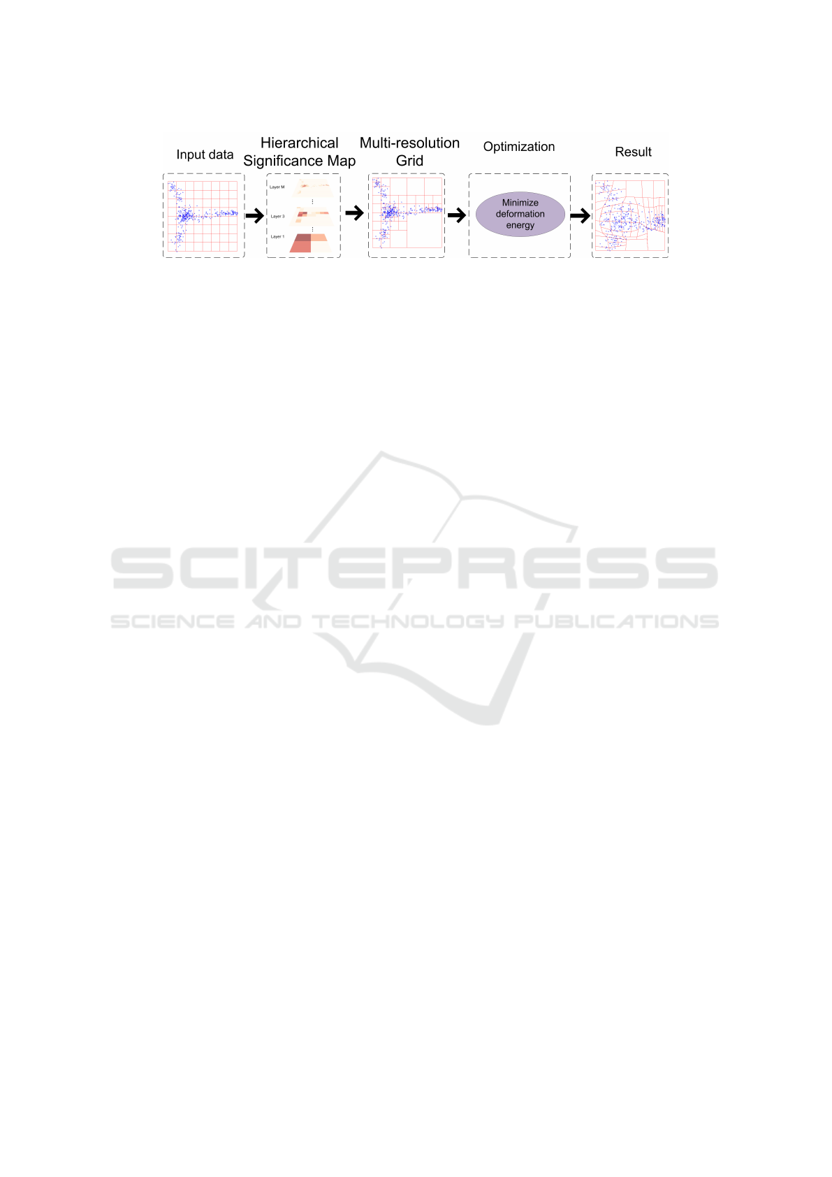
Figure 1: Method overview: The ﬁrst step is the generation of hierarchical signiﬁcance map. Afterwards the multi-resolution

grid is generated and the optimization is applied onto this grid based on the hierarchical signiﬁcance map in order to identify

its optimal deformation. The result is a deformed visualization space which enhances cluttered areas on the display. An HR

copy of this Figure can be found in the following link http://www.iti.gr/

∼

drosou/HierarchicalMagniﬁcation/Fig1.jpg.

dividual layer, for the subsequent superposition of the

maps. The operator ℵ(.) deﬁned in (Itti et al., 1998)

is utilized so as to normalize each signiﬁcance map.

The same normalization operator ℵ(.) has also

been used in other research works (e.g. (Jia et al.,

2014) and (Lee et al., 2005)), and has as a result the

promotion of signiﬁcance maps, which are comprised

of a small number of high signiﬁcance values, while

efﬁciently suppressing signiﬁcance maps with a large

number of similar values.

The ﬁnal hierarchical signiﬁcance map is created

for the resolution of the last layer of the grid hier-

archy G

. To achieve this, let us denote as Q





where l is the level of the hierarchy and f

∈ F

is a

speciﬁc hyperrectangle belonging to layer l, as the set

of hyperrectangles from all the layers of the hierar-

chy, so that they intersect with the N-dimensional hy-

perrectangle f

. In the speciﬁc case of this paper that

= 2

partitions per dimension are considered, if two

hyperrectangles intersect, it means that one contains

the other. The same stands true for every n

= r

for

r ∈ N

. In the same notion Q





is the set of sig-

niﬁcance values of all the hyperrectangles belonging

to Q





. The superpositioning of the different maps

is performed on layer M and the ﬁnal hierarchical sig-

niﬁcance map, denoted as S

hier

, is calculated for each

hyperrectangle in layer M. Let s

be the ﬁnal hierar-

chical signiﬁcance value of hyperrectangle f

∈ F

The calculation of s

is described in Eq.(1)

hier

∑

∈Q

(

)

ℵ





(1)

Finally, the hierarchical signiﬁcance map is de-

ﬁned as S

hier

3.2 Multi-resolution Grid

The multi-resolution grid is a non-uniform grid on the

N-dimensional space, in which the distribution of hy-

perrectangles is not uniform, but instead distributes

more hyperrectangles in regions with high signiﬁ-

cance. The advantage of the multi-resolution grid is

that regions with high signiﬁcance are less distorted

when magniﬁed, since they have higher resolution.

In addition the optimization space of the vertex po-

sitions of the grid is much smaller when compared to

the full resolution grid, and thus, has better speed per-

formances and also produces better results (as shown

in Section 4.1).

The algorithm for the creation of the multi-

resolution grid is similar to the one used for the cre-

ation of a quad tree. The algorithm takes as input a

speciﬁc user-deﬁned signiﬁcance threshold. In the

context of this work this threshold is set to a value that

results in the reduction of the number of optimization

variables by 20% to 50%, depending on the appli-

cation. This algorithm has as a result, that the sig-

niﬁcance value of each hyperrectangle is the largest

possible value, which is smaller than the provided

threshold (i.e. the inﬁmum). The multi-resolution

grid is denoted as G

mul

, E

mul

, F

mul

), where F

mul

are hyperrectangles of the multi-resolution grid, V

mul

the vertices and E

mul

the edges.

The signiﬁcance value s

mul

of each hyperrectangle

mul

∈ F

mul

in the multi-resolution grid is calculated

from the hierarchical signiﬁcance map S

hier

deﬁned in

Section 3.1. For this calculation, the values of hierar-

chical signiﬁcance map S

hier

have to be mapped on the

hyperrectangles in F

mul

. As explained in Section 3.1,

the hierarchical signiﬁcance map S

hier

is deﬁned for

each hyperrectangle of the grid G

in the maximum

layer of the grid hierarchy layer M.

Let P( f

mul

) denote the set of all hyperrectan-

gles from grid G

, which intersect with f

mul

∈ F

mul

Additionally, let P

( f

mul

) denote the set of signiﬁ-

cance values of all the hyperrectangles belonging to

P( f

mul

). The procedure of calculation of the signiﬁ-

cance value of each hyperrectangle f

mul

∈ F

mul

in the

multi-resolution grid G

mul

is deﬁned in Eq.(2).

IVAPP 2017 - International Conference on Information Visualization Theory and Applications

mul

∑

∀s

hier

∈P

(

mul

)

hier

(2)

The signiﬁcance map of the multi-resolution grid

mul

is deﬁned as S

mul

. The algorithm for

the computation of the multi-resolution grid can be

found in the following link http://www.iti.gr/

∼

drosou/

HierarchicalMagniﬁcation/multiResGrid.png.

3.3 Grid Deformation Procedure

This section follows the work presented in (Wang

et al., 2008) and (Wu et al., 2013), regarding the grid

deformation procedure. The deformation procedure

presented here has been ﬁrstly proposed by (Wang

et al., 2008) for image resizing. The same proce-

dure has afterwards been utilized by (Wu et al., 2013)

for resizing data visualizations. More details can be

found in (Wang et al., 2008) and (Wu et al., 2013).

The purpose of grid deformation is to enlarge sig-

niﬁcant regions of the input space, and visualize any

patterns that were previously hidden due to high clut-

tering. The deformation method takes as input a grid

G = (V, E, F) and its signiﬁcance map S, where V

the matrix of vertices, E matrix of edges, and F the

matrix of hyperrectangles. These matrices have spe-

ciﬁc relationships between them, i.e. F = QV and

E = HV , where Q and H are also matrices which de-

pend on the grid. The result of deformation is a new

grid G



, E

, F



, created by changing the posi-

tions of the vertices in V , according to the given sig-

niﬁcance map.

According to (Wang et al., 2008) and (Wu et al.,

2013), the ideal deformation of each v

∈V into a new

position should be deﬁned as v

= c ∗v

, where c is the

scale factor. This equation refers to the uniform scal-

ing case, and requires an extension of the area covered

by the data in the input space. In the case that the area

covered by the data in the input space is considered

static, then the enlargement is not possible. One of

the alternatives proposed in the literature (see Section

2) is to introduce a non-linear deformation of each hy-

perrectangle, so that more space is given to more sig-

niﬁcant hyperrectangles (Wang et al., 2008)(Wu et al.,

2013).

The main objective of the utilized grid defor-

mation method is to minimize the total deformation

energy, deﬁned as the distance from the uniformly

scaled position. Let f

∈ F be a hyperrectangle de-

ﬁned as f

= q

V , where q

is a 2

×|V | matrix (N is

the dimension) and its element in the r

row and c

column is deﬁned as:

i,rc



1 , i f v

∈ f

, and f

i,r

= v

0 , else



(3)

where f

, r is the r

vertex in f

. Given Q =

, q

, ...., q

|F|

, the matrix of hyperrectangles is

deﬁned as F = QV .

The uniformly scaled hyperrectangle is deﬁned as

= c

, where c

is the desired scale matrix for the

h hyperrectangle. Let F

= [ f

, f

, .., f

|F|

] be a ma-

trix of all the quads, and W

be a |F|×|F| matrix of

the signiﬁcance of each quad, while its element in the

row and c

column is deﬁned as:

F,rc



√

, i f r = c

0 , else



(4)

where s

is the signiﬁcance of hyperrectangle f

. Fur-

thermore, let C be the desired scale matrix C with:



, i f r = c

0 , else



(5)

The total hyperrectangle deformation energy is

deﬁned in Eq.(6)



−W



−W

CQV



(6)

The minimization of the total hyperrectangle de-

formation energy allows for the hyperrectangles with

large signiﬁcance, to have a smaller distance from

their uniformly scaled version (which refers to the

lack of distortion for all the objects), and thus, under

the constraint of static space, signiﬁcant hyperrectan-

gles are enlarged more than less signiﬁcant ones.

An additional energy term that is used for the de-

formation procedure is the edge bending, as proposed

in (Wu et al., 2013) and (Wang et al., 2008).

Given an edge e

, its uniformly scaled version is

deﬁned as e

= l

, where l

is a 2 ×2 scale matrix.

Let E

= [e

, e

, .., e

|E|

] be a matrix of all the edges,

and W

be a |E|×|E| matrix of the signiﬁcance of

each edge, while its element in the r

row and c

column is deﬁned as:

E,rc



√

, i f r = c

0 , else



(7)

where s

is the average signiﬁcance factor for all the

hyperrectangles in which edge e

belongs. Further-

more, let L be the desired scale matrix L with:



, i f r = c

0 , else



(8)

The total edge bending energy is deﬁned as



−W



−W

LHV



(9)

where H is a matrix such that E = HV . The edge

bending energy term scales the edge lengths and tries

A Hierarchical Magniﬁcation Approach for Enhancing the Insight in Data Visualizations

to retain the edge orientations, after the grid deforma-

tion.

Finally, the optimum deformed grid is deﬁned as

a solution to the following minimization problem:

argmin



(QV

−CQV )



(HV

−LHV )



(10)

subject to the following constraints:











i,d

= min[d] , i f v

i,d

is on the lower

boundary o f dimention d

i,d

= max[d] , i f v

i,d

is on the upper

boundary o f dimention d











where v

i,d

is the coordinate of vertex v

∈V in the d

dimension, and min [d] and max[d] are the lower and

upper boundaries of the d

dimension as deﬁned by

the input dataset. After the minimization of the to-

tal deformation energy D deﬁned in Eq.(10), the new

grid G



, E, F



is found, where V

. The

dataset is deformed to this new grid G

, taking the

initial grid into account G and utilizing linear interpo-

lation in the one/two/three-dimensional space.

At this point it should be mentioned that that the

proposed method illustrates the objects (e.g. graphs,

wordclouds, etc.) to be magniﬁed, via the processing

of their corresponding signiﬁcancies at certain time-

instances. In this context, a direct comparison be-

tween different time-instances, would be rather prone

to inconsistencies. Moreover, the reader should note

that the deformation grid depicted in most of the ﬁg-

ures, is used for demonstration purposes, while it

would be meaningful in illustration cases where a

comparison to the original shape of the magniﬁed ob-

ject is wanted.

4 EXPERIMENTAL RESULTS

This section presents the application of the Magniﬁca-

tion approach to the following different visualization

approaches: 1) Word clouds, 2) Scatterplots, and 3)

Choropleth maps.

4.1 Evaluation Metrics

4.1.1 Pattern Preservation

The Pattern Preservation (PP) evaluation metric cap-

tures the degree in which the local regions in the mag-

niﬁed space preserve the patterns that existed in the

input space. This metric is based on graph match-

ing on the kNN (k-Nearest Neighbors) graphs be-

tween the input and magniﬁed spaces (example of

this metric is presented in (Hautam

aki et al., 2008)).

Graph representations of the input data, and subse-

quent graph matching, have been used in the liter-

ature for the comparison of 3D objects and point

clouds (e.g. (Hilaga et al., 2001)(Tung and Schmitt,

2005)(Mademlis et al., 2008)), as well as for speaker

identity recognition (e.g. (Hautam

aki et al., 2008)).

A large change in the number of neighbors for each

data instance represents a large change of the ini-

tial pattern due to the magniﬁcation procedure. The

graph matching distance is found using the graph edit

distance(Gao et al., 2010) between the labeled kNN

graphs of the input and magniﬁed spaces.

4.1.2 Size Perception

The Size Perception (SP) evaluation metric attempts

to quantify the humans’ visual perception of different

sizes of objects. Equivalently with most of the human

senses, the human perception of an external stimuli is

not linearly proportional to the intensity of the stim-

uli. For instance, acousticians say that doubling of the

volume (loudness) should be sensed as a level differ-

ence of +10dB.

Similarly, the SP metric captures a signiﬁcant an-

alytical task, the degree in which the resizing factor

of the objects is correctly perceived in the magniﬁed

space. In this respect, the Stevens’ Power Law (Zwis-

locki, 2009) has been utilized, according to which the

perception of the intensity of a sensory stimuli is a

power function of the actual intensity of the stimuli

(i.e. ψ(I) = kI

, whereby I is the intensity of the input

stimuli, ψ(I) is the subjective magnitude of the sen-

sation, a is an exponent that depends on the sensory

type of the stimulation, and k a constant). According

to Brewer et al. (Brewer, 1994) k = 0.98 and a = 0.87,

when size perception is regarded.

The proposed evaluation metric measures the ab-

solute difference of the actual input size, from the size

perceived by the visualization: SP =

∑

ψ(I

) −L

where ψ(I

) is the perceived size of the i

visual ob-

ject, and L

its intended size as speciﬁed from the in-

put data.

4.1.3 Jensen−Shannon divergence

The Jensen−Shannon Divergence (JSD) (Endres

and Schindelin, 2003) is used in probability the-

ory in order to measure the distance between two

one-dimensional distributions. It is based on the

Kullback−Leibler divergence(Endres and Schindelin,

IVAPP 2017 - International Conference on Information Visualization Theory and Applications

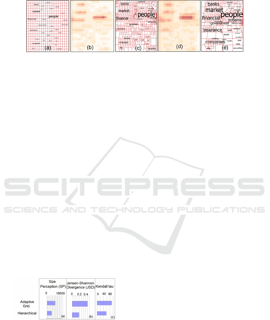
Figure 2: Results of the application of the Magniﬁcation approach on the word cloud visualization with magniﬁcation factor

equal to 4. (a) Input visualization (b) Single layer signiﬁcance map proposed in (Wu et al., 2013). (c) Results obtained from

the single layer signiﬁcance map (in (b)). (d) Hierarchical signiﬁcance map generated from the saliency based signiﬁcance

map proposed in (Wu et al., 2013). (e) Result obtained from the hierarchical signiﬁcance map (in (d)). The proposed approach

in (e), takes better advantage of the empty space, and enlarges more the words of the visualization. An HR copy of this Figure

can be found in the following link http://www.iti.gr/

∼

drosou/HierarchicalMagniﬁcation/Fig2.jpg.

2003), and is a symmetric metric.

4.2 Word Clouds

In this experiment, the efﬁciency of the proposed

multi-resolution magniﬁcation approach is demon-

strated on the word clouds visualization.

The resizing of the word cloud in smaller screens

can cause cluttering. The most common reason for

this type of cluttering is that some words can be-

come very small to read/understand, which unavoid-

ably leads to information loss. High cluttering is

also caused by not preserving the relative sizes of the

words in the deformed space. In order to solve this is-

sue, we utilize non-linear deformation that increases

the size of the words, while also preserving the rela-

tive sizes of the words. The increase in the size of the

words is performed in such a way (through the use of

the signiﬁcance map and the deformation procedure),

so as to preserve the relative sizes of the words as

much as possible, and thus, have a minimum change

in the relationship between different words. Hence,

the size of the words in the magniﬁed space is (al-

most) proportional to the size of the words in the input

space.

Figure 3: The evaluation results using the SP (a) and JSD

(b) and Kendall tau (c) metrics applied on Figure 2(c), and

Figure 2(e) respectively. Smaller values represent better re-

sults. The hierarchical approach provides the best results in

all the metrics.

In this context, each word is considered as a vi-

sual item, which is attached on all the grid cells that

contain it. After the grid deformation, the position

of the words is adjusted by means of interpolation,

while the ﬁnal word resizing is found from the as-

sociated cell deformations. In addition, in order to

avoid word overlapping, a collision avoidance algo-

rithm which can change the positions of the words in

case of collision was implemented.

In this experiment, a context-preserving word

cloud by a force-directed algorithm (Cui et al., 2010)

was used on a real dataset with 13,828 news arti-

cles spanning one year (from 2008 to 2009) that were

related to American International Group (AIG). The

context-preserving word cloud results in positioning

semantically-similar words close to each other.

Figure 2 presents the results of applying the pro-

posed Magniﬁcation approach on the aforementioned

word cloud visualization. Figure 2(a) shows the input

data. Figure 2(b) and Figure 2(d) illustrate the single

layer and hierarchical signiﬁcance maps respectively,

generated using the signiﬁcance map proposed in (Wu

et al., 2013) as a base. As shown in these ﬁgures, the

hierarchical signiﬁcance map is smoother around sig-

niﬁcant regions. The corresponding results of each of

these maps are shown in Figure 2(c) and Figure 2(e),

in which the ﬁrst utilizes the single layer signiﬁcance

map, while the latter utilizes the hierarchical signiﬁ-

cance map. Figure 2(e) utilizes better the empty space

for the magniﬁcation of the words, and produces bet-

ter results.

Figure 3 presents the evaluation results applied

on Figure 2, using the SP and JSD evaluation met-

rics presented in Section 4.1, as well as the Kendal

tau distance metric presented in the next paragraphs.

The SP metric shows that the multi-resolution grid has

the smallest distance between the perception of the

sizes of the words, and their intented size, and thus,

it is more perceptually consistent. The JSD metric

is used to compare the normalized distribution of the

sizes of the words in the input word cloud with re-

spect to the word sizes in the deformed spaces. The

proposed approach provides the better results. A ﬁg-

A Hierarchical Magniﬁcation Approach for Enhancing the Insight in Data Visualizations

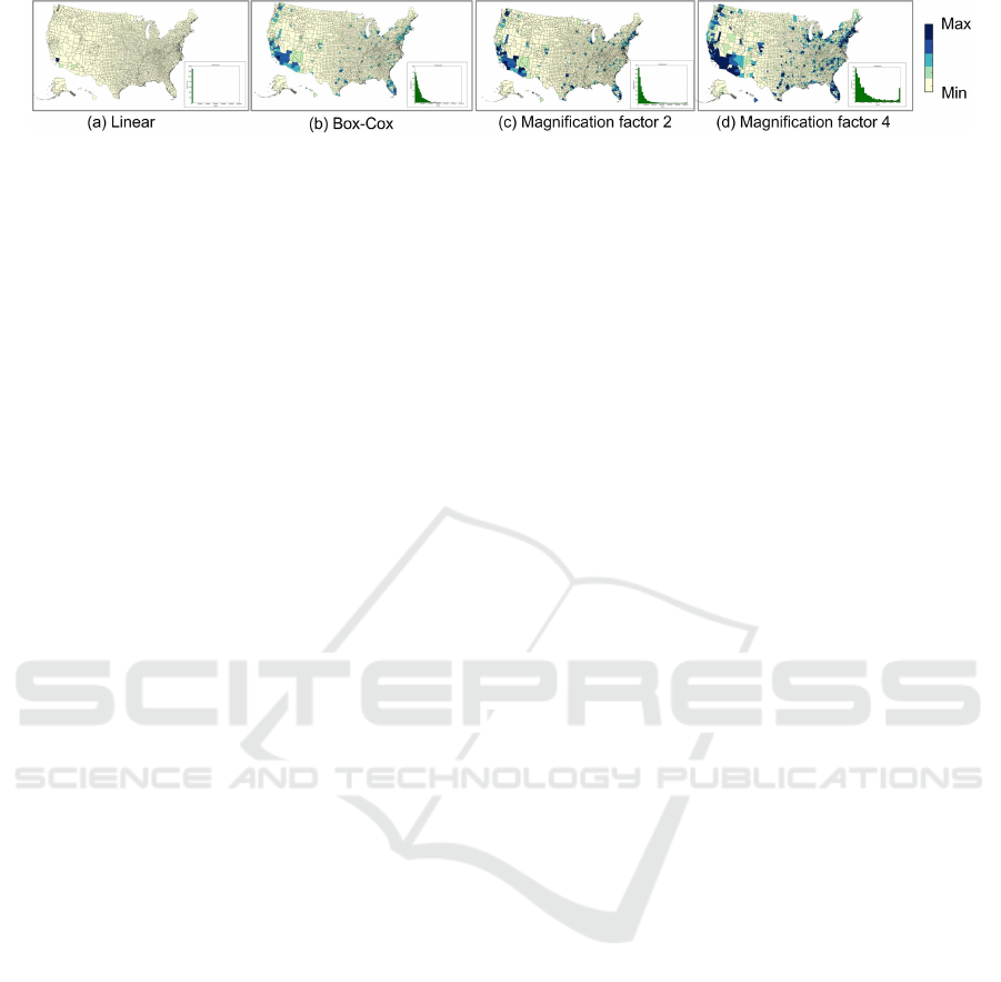
Figure 4: Results of the application of the Magniﬁcation approach on a choropleth map, visualizing the unemployment

data for each US area in 2011. The lower right part of each subﬁgure shows the corresponding distribution. (a) Lineal

mapping. (b) Box-Cox mapping(Maciejewski et al., 2013). (c) Magniﬁcation factor equal to 2. (d) Magniﬁcation factor

equal to 4. Although subﬁgure (d) loses some information regarding the high values of the dataset, it provides more color

resolution to the lower ranges of the data (where the majority of the data values lies), and thus, small differences between

the different states are better visualized and perceived. An HR copy of this Figure can be found in the following link http:

//www.iti.gr/

∼

drosou/HierarchicalMagniﬁcation/Fig4.jpg.

ure that shows the normalized distributions can be

found in the following link http://www.iti.gr/

∼

drosou/

HierarchicalMagniﬁcation/normDistr.png.

In order to measure how the relative sizes of the

words change, after the application of each defor-

mation method, we utilize the Kendall tau distance

(Fagin et al., 2003). This is a distance metric be-

tween two ordered lists. In this case the ﬁrst or-

dered list is the list of sizes of the input words, and

the second is the list of words in the magniﬁed re-

sult. Figure 3(c) shows the results of this metric.

Smaller values represent a greater preservation of

the relative ordering of the sizes in the words. The

smallest Kendall tau distance is obtained by the pro-

posed hierarchical approach. A ﬁgure that shows

how the ordered lists change for each method can be

found in the following link http://www.iti.gr/

∼

drosou/

HierarchicalMagniﬁcation/wordsOrder.png.

4.3 Scatterplots

This section presents the application of the Magniﬁ-

cation approach on scatterplot visualizations. Each

point in the scatterplot is attached to a speciﬁc hy-

perrectangle of the grid. After the magniﬁcation pro-

cedure, the new point positions are found by means

of interpolation on the new hyperrectangle positions.

The size of the points does not change.

For the generation of the scatterplots, the data

from INSPIRE (Wong and Thomas, 2009) is used.

These data reveal the topic distribution of IEEE Vis,

IEEE InfoVis and, IEEE VAST proceeding papers

published from 2006 to 2008.

Figure 5 presents the results of the application of

the magniﬁcation approach on the scatterplot visual-

ization of the aforementioned INSPIRE dataset. Two

types of signiﬁcance maps were utilized, the entropy

and saliency(Wu et al., 2013) maps, using both one

layer and hierarchical signiﬁcance deﬁnition. The hi-

erarchical signiﬁcance map takes better advantage of

the empty space, and enlarges the signiﬁcant areas

more, with minimum deformation of the local pattern

distribution.

The values of the PP evaluation metric applied on

Figure 5 are shown in Figure 6. Since the size of the

points in the scatterplot remains the same after the

magniﬁcation procedure, only the PP metric is used.

This ﬁgure reveals that the best results are obtained

from the hierarchical grid approach proposed in this

work, using the saliency-based signiﬁcance map pro-

posed in (Wu et al., 2013).

Figure 7 presents an example of application of

the Magniﬁcation approach on a 3D scatterplot vi-

sualization using the forest ﬁres dataset(Cortez and

Morais, 2007), which contains meteorological data

from burned forests in the northeast region of Por-

tugal. Speciﬁcally, the Fine Fuel Moisture Code

(FFMC), Drought Code (DC), and the Initial Spread

Index (ISI), are used for the generation of the scatter-

plot. The hierarchical grids for the initial and magni-

ﬁed scatterplots are shown in Figure 7(a) and Figure

7(b), using entropy signiﬁcance map, while the cor-

responding magniﬁcation results are shown in Figure

7(c) and Figure 7(d). The correlations between the

visualized variables, which are hidden in the initial

view due to high cluttering, are visualized better in

the magniﬁed result.

4.4 Choropleth Maps

This section presents the application of the Mag-

niﬁcation approach on choropleth maps, in which

color is utilized to encode quantitative information.

In this visualization, each area of the map has a

speciﬁc attribute value which is mapped on to its

color. The magniﬁcation approach is applied on the

1-dimensional input dataset, and afterwards, the mag-

niﬁed space is mapped onto the color values. For this

visualization the unemployment of 2011 from the US

Census (Census, 2014) dataset is used.

Figure 4 presents the results of the Magniﬁca-

tion approach on the choropleth map. Figure 4(a)

presents the case of linear mapping, Figure 4(b) the

Box-Cox transformation proposed by (Maciejewski

IVAPP 2017 - International Conference on Information Visualization Theory and Applications

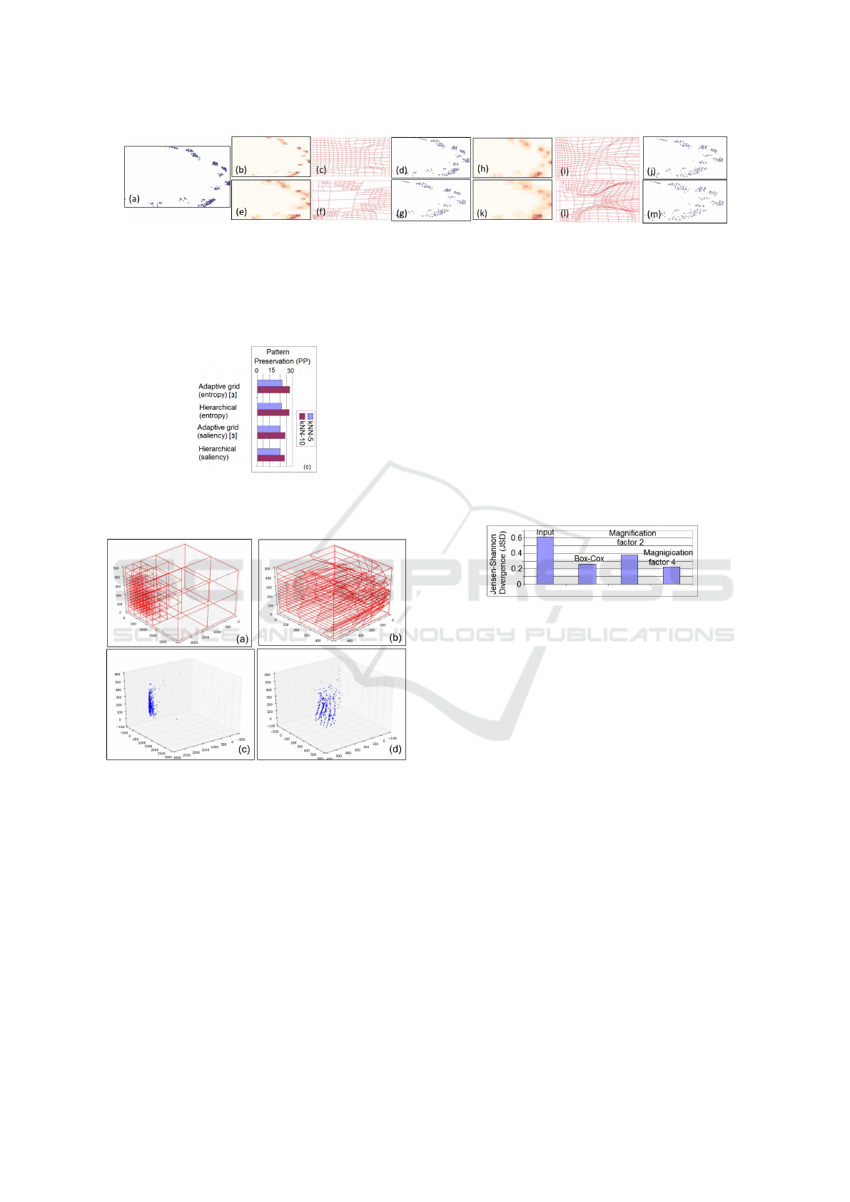
Figure 5: Results of the application of the Magniﬁcation approach on a scatterplot visualization with magniﬁcation factor

equal to 3. (a) Input visualization. (b),(e) Single layer and hierarchical signiﬁcance maps generated using the entropy of each

hyperrectangle. (c),(d),(f),(g) Results of the signiﬁcance maps shown in (b) and (e) using the method proposed in (Wu et al.,

2013) and in this paper respectively. (h),(k) Single layer and hierarchical signiﬁcance maps generated from the saliency based

signiﬁcance map proposed in (Wu et al., 2013). (i),(j),(l),(m) Results of the signiﬁcance maps shown in (h) and (k) using the

method proposed in (Wu et al., 2013) and in this paper respectively. An HR copy of this Figure can be found in the following

link http://www.iti.gr/

∼

drosou/HierarchicalMagniﬁcation/Fig5.jpg.

Figure 6: PP metric for Figure 5. The smaller the value

the better the results. The best results are obtained from

proposed approach using a saliency signiﬁcance map.

Figure 7: Application of the Magniﬁcation approach

on a 3D scatterplot visualization using the forest ﬁres

dataset(Cortez and Morais, 2007). An HR copy of this

Figure can be found in the following link http://www.iti.gr/

∼

drosou/HierarchicalMagniﬁcation/Fig7.jpg.

et al., 2013), while Figure 4(c) and Figure 4(d) present

the results with a magniﬁcation factor manually se-

lected to be equal to 2 and 4 respectively. The right

lower part of the ﬁgures shows the histogram of the

distribution of the data in each case.

In the case of linear mapping shown in Figure

4(a), due to the fact that the distribution is very

skewed towards zero, most of the information is clut-

tered and is not visualized. On the other hand, the

visualization on Figure 4(c) and Figure 4(d) is more

uniformly distributed, and the choropleth map shows

more information regarding the status of the civilian

labor force to the different areas of the US. It should

be noted that the results and distribution of the data

for the (Maciejewski et al., 2013) mapping resemble

the results of the magniﬁcation approach for a magni-

ﬁcation factor equal to 4. The visualization in Figure

4(d) provides more information regarding the distri-

bution of the data in the lower ranges of its values,

and the small differences between the different states

are more evident.

Figure 8: The JSD metric measures the distance of the color

distribution created from the deformation methods in Fig-

ure 4, from the optimum uniform distribution (according to

(Brewer and Pickle, 2002)). Using a magniﬁcation factor

equal to 4, the results are better than Box-Cox mapping.

For the evaluation of the deformation results in

Figure 4, the work presented by Brewer and Pickle

(Brewer and Pickle, 2002) is used. Speciﬁcally,

Brewer and Pickle contacted multiple user studies

in order to evaluate the effectiveness of the different

color mapping techniques in choropleth maps, and in-

vestigate how they affected user performance in vari-

ous tasks. They found that the best mapping method is

the quantile mapping, which assigns the same number

of data objects to each of the available colors. This is

in fact a uniform distribution in the color plane. Tak-

ing this fact into account, the use of the JSD metric is

used to measure the distance of the distribution of the

colors created by the deformation procedure, from the

optimum uniform distribution.

The results of the JSD metric are presented in Fig-

ure 8, which show that increasing of the magniﬁcation

factor results in more uniform distributions, and thus,

better results. Using magniﬁcation factor equal to 4,

the results are better than Box-Cox mapping.

A Hierarchical Magniﬁcation Approach for Enhancing the Insight in Data Visualizations

4.5 User Evaluation Results

This section presents the results of the user evalua-

tion studies. The participants were presented with

a variety of visualization methods that were magni-

ﬁed utilizing either the proposed magniﬁcation ap-

proach, or other state-of-the-art methods. The appli-

cations considered resizing/magniﬁcation of: scatter-

plot, word cloud and color (in choropleth maps). In

the case of scatterplot and word cloud magniﬁcation,

the approach proposed by Wu et al. (Wu et al., 2013)

was used for comparison. In the case of the choro-

pleth map, the Box-Cox mapping (Maciejewski et al.,

2013) has been used for comparison with the pro-

posed approach. For the evaluation studies, the same

datasets presented in this paper were utilized.

Three visualizations were given for each applica-

tion, the input visualization, and the two result vi-

sualizations (produced by applying the proposed ap-

proach and the other state-of-the-art method respec-

tively). The participants were asked to select one of

the result visualization. The following questions were

asked to the participants depending on the applica-

tion:

• In the scatterplot and word cloud applica-

tion: Which result provides better understand-

ing/insight about the input visualization?

• In the choropleth map application: Which result

represents more information about the input data?

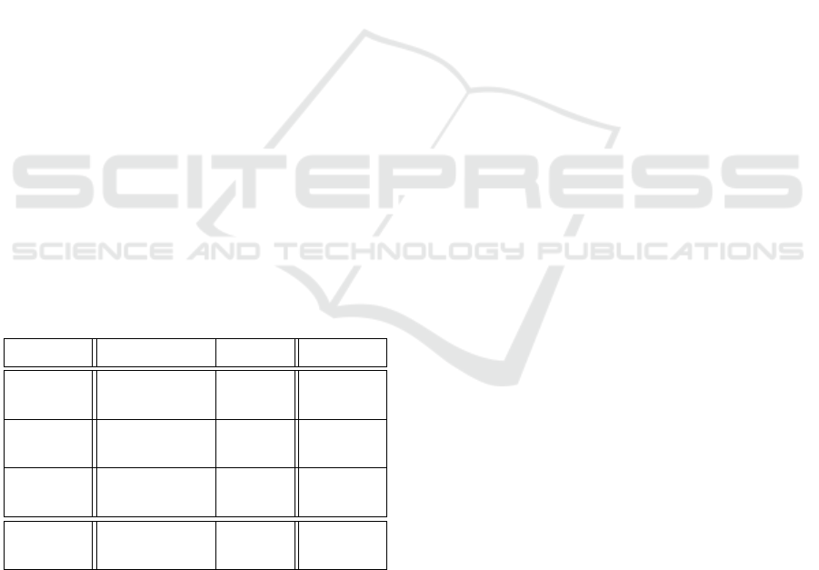
Table 1: The results of the user evaluation studies on 22

individuals. The participants had to select between the pro-

posed hierarchical approach and other state-of-the-art meth-

ods.

Hierarchical Other p-val

Scatter-

plot

63.64% 36.36% 0.2008

Choro-

pleth

95.45% 4.55% 0.00002

Word-

cloud

81.82% 18.18% 0.0028

Overall 80.03% 19.69% 1.522e-

The results of the user evaluation studies are illus-

trated in Table 1. As shown in this ﬁgure, the par-

ticipants selected the results of hierarchical approach

more often than the competing method. The differ-

ence is larger in the choropleth map and word cloud

visualizations. Smaller difference can be found in the

scatterplot application. General discussion with the

users after the evaluation revealed two distinct groups.

The ﬁrst group preferred displays with dense clusters,

that had a large distance between them, and this is

the reason they selected the less magniﬁed result (i.e.

the competing method in (Wu et al., 2013), since the

magniﬁcation using the hierarchical method was gen-

erally larger). On the other hand, the second group

found that the more magniﬁed view provided better

insight regarding the ﬁne details within a cluster. Ta-

ble 1 also presents the results of hypothesis testing,

i.e. chi-square goodness of ﬁt, in order to identify

the difference of the observed distributions with re-

spect to random guess. In all the cases except for the

scatterplot visualization, the results are indeed statis-

tically signiﬁcant. Overall, 80.03% of the participants

selected the hierarchical approach with p-value below

0.005.

5 CONCLUSIONS

This work introduces a hierarchical magniﬁcation ap-

proach that enables the interactive reduction of vi-

sual clutter, and the magniﬁcation of signiﬁcant re-

gions of the data in multiple dimensions. Signiﬁcant

regions are uniformly magniﬁed with minimum dis-

tortion, while the distortion is distributed to the less

signiﬁcant areas of the display. This is particularly

useful for visualization resizing to ﬁt small screens.

The proposed hierarchical signiﬁcance map com-

bines the information of the signiﬁcance maps over

multiple grid scales, based on each hyperrectangle’s

intersections with other hyperrectangles, and the sig-

niﬁcance of each grid using a normalization operator.

The proposed approach identiﬁes both small and large

objects/patterns, and scales them with minimum dis-

tortion in the magniﬁed space. In addition, the intro-

duction of the multi-resolution grid reduces the num-

ber of variables in the optimization space, and thus,

decreases the running time of the algorithm.

The efﬁciency of the proposed approach was

demonstrated on multiple visualization approaches,

and the results were found to be superior to previous

methods using multiple evaluation metrics and user

studies.

The main advantage of the proposed approach is

that it does not address speciﬁc application areas. The

proposed approach can be used in order to enhance

any type of signiﬁcance map, but the exact choice of

the signiﬁcance map depends on the application.

Future work includes the research of additional

irregular grid formations (e.g. non-rectangular grids

based on edge detection algorithms), and their effect

on the distortion after the optimization procedure. Al-

ternative signiﬁcance maps will also be considered,

IVAPP 2017 - International Conference on Information Visualization Theory and Applications

since an important aspect of the future work includes

the automatic selection of the most appropriate signif-

icance map based on the input dataset.

ACKNOWLEDGMENT

This work has been partially supported by the Euro-

pean Commission through project Scan4Reco funded

by the European Union H2020 programme under

Grant Agreement n

665091. The opinions expressed

in this paper are those of the authors and do not neces-

sarily reﬂect the views of the European Commission.

REFERENCES

Bertini, E. and Santucci, G. (2006). Give chance a

chance: Modeling density to enhance scatter plot

quality through random data sampling. Information

Visualization, 5(2):95–110.

Brewer, C. A. (1994). Cartography: thematic map design.

Cartographic Perspectives, (17):26–27.

Brewer, C. A. and Pickle, L. (2002). Evaluation of meth-

ods for classifying epidemiological data on choropleth

maps in series. Annals of the Association of American

Geographers, 92(4):662–681.

Census (2014). US Census Bureau (available at

http://www.census.gov/).

Cortez, P. and Morais, A. d. J. R. (2007). A data mining

approach to predict forest ﬁres using meteorological

data.

Cover, T. M. and Thomas, J. A. (2012). Elements of infor-

mation theory. John Wiley & Sons.

Cui, W., Wu, Y., Liu, S., Wei, F., Zhou, M. X., and Qu, H.

(2010). Context preserving dynamic word cloud vi-

sualization. In Paciﬁc Visualization Symposium (Paci-

ﬁcVis), 2010 IEEE, pages 121–128. IEEE.

Eisemann, M., Albuquerque, G., and Magnor, M. (2011).

Data driven color mapping. Proceedings EuroVA.

Ellis, G. and Dix, A. (2007). A taxonomy of clutter

reduction for information visualisation. Visualiza-

tion and Computer Graphics, IEEE Transactions on,

13(6):1216–1223.

Endres, D. M. and Schindelin, J. E. (2003). A new met-

ric for probability distributions. Information Theory,

IEEE Transactions on, 49(7):1858–1860.

Fagin, R., Kumar, R., and Sivakumar, D. (2003). Compar-

ing top k lists. SIAM Journal on Discrete Mathemat-

ics, 17(1):134–160.

Gao, X., Xiao, B., Tao, D., and Li, X. (2010). A survey of

graph edit distance. Pattern Analysis and applications,

13(1):113–129.

Hautam

aki, V., Kinnunen, T., and Fr

anti, P. (2008). Text-

independent speaker recognition using graph match-

ing. Pattern Recognition Letters, 29(9):1427–1432.

Hilaga, M., Shinagawa, Y., Kohmura, T., and Kunii, T. L.

(2001). Topology matching for fully automatic simi-

larity estimation of 3D shapes. In Proceedings of the

28th annual conference on Computer graphics and in-

teractive techniques, pages 203–212. ACM.

Itti, L., Koch, C., and Niebur, E. (1998). A model of

saliency-based visual attention for rapid scene anal-

ysis. IEEE Transactions on pattern analysis and ma-

chine intelligence, 20(11):1254–1259.

Jia, S., Zhang, C., Li, X., and Zhou, Y. (2014). Mesh resiz-

ing based on hierarchical saliency detection. Graphi-

cal Models.

Keim, D. A., Hao, M. C., Dayal, U., Janetzko, H., and Bak,

P. (2010). Generalized scatter plots. Information Vi-

sualization, 9(4):301–311.

Lee, C. H., Varshney, A., and Jacobs, D. W. (2005). Mesh

saliency. In ACM Transactions on Graphics (TOG),

volume 24, pages 659–666. ACM.

Maciejewski, R., Pattath, A., Ko, S., Hafen, R., Cleveland,

W. S., and Ebert, D. S. (2013). Automated box-cox

transformations for improved visual encoding. Visu-

alization and Computer Graphics, IEEE Transactions

on, 19(1):130–140.

Mademlis, A., Daras, P., Axenopoulos, A., Tzovaras, D.,

and Strintzis, M. G. (2008). Combining topological

and geometrical features for global and partial 3-D

shape retrieval. Multimedia, IEEE Transactions on,

10(5):819–831.

Rosenholtz, R., Li, Y., Mansﬁeld, J., and Jin, Z. (2005).

Feature congestion: a measure of display clutter. In

Proceedings of the SIGCHI conference on Human fac-

tors in computing systems, pages 761–770. ACM.

Tao, J., Wang, C., Shene, C.-K., and Kim, S. H. (2014).

A Deformation Framework for Focus+Context Flow

Visualization. Visualization and Computer Graphics,

IEEE Transactions on, 20(1):42–55.

Thompson, D., Bennett, J., Seshadhri, C., and Pinar, A.

(2013). A provably-robust sampling method for gen-

erating colormaps of large data. In Large-Scale Data

Analysis and Visualization (LDAV), 2013 IEEE Sym-

posium on, pages 77–84. IEEE.

Tung, T. and Schmitt, F. (2005). The Augmented Multires-

olution Reeb Graph Approach for Content-based Re-

trieval of 3d Shapes. International Journal of Shape

Modeling, 11(1):91–120.

Wang, Y.-S., Tai, C.-L., Sorkine, O., and Lee, T.-Y. (2008).

Optimized scale-and-stretch for image resizing. In

ACM Transactions on Graphics (TOG), volume 27,

page 118. ACM.

Wang, Y.-S., Wang, C., Lee, T.-Y., and Ma, K.-L. (2011).

Feature-preserving volume data reduction and focus+

context visualization. Visualization and Computer

Graphics, IEEE Transactions on, 17(2):171–181.

Wong, P. C. and Thomas, J. (2009). Visual analytics: build-

ing a vibrant and resilient national science. Informa-

tion Visualization, 8(4):302–308.

Wu, Y., Liu, X., Liu, S., and Ma, K.-L. (2013). Vi-

Sizer: a visualization resizing framework. Visualiza-

tion and Computer Graphics, IEEE Transactions on,

19(2):278–290.

Zwislocki, J. J. (2009). Stevens’ Power Law. Sensory Neu-

roscience: Four Laws of Psychophysics, pages 1–80.

A Hierarchical Magniﬁcation Approach for Enhancing the Insight in Data Visualizations