
A Semi-local Surface Feature for Learning Successful Grasping
Affordances
Mikkel Tang Thomsen, Dirk Kraft and Norbert Kr
¨
uger
Maersk Mc-Kinney Moller Institute, University of Southern Denmark, Campusvej 55, 5230, Odense M, Denmark
Keywords:
Computer Vision, Robotics, Grasp Affordance Learning.
Abstract:
We address the problem of vision based grasp affordance learning and prediction on novel objects by proposing
a new semi-local shape-based descriptor, the Sliced Pineapple Grid Feature (SPGF). The primary characteristic
of the feature is the ability to encode semantically distinct surface structures, such as “walls”, “edges” and
“rims”, that show particular potential as a primer for grasp affordance learning and prediction. When the
SPGF feature is used in combination with a probabilistic grasp affordance learning approach, we are able to
achieve grasp success-rates of up to 84% for a varied object set of three classes and up to 96% for class specific
objects.
1 INTRODUCTION
An important problem that is being addressed in com-
puter vision and robotics is the ability for agents to
interact in previously unseen environments. This is a
challenging problem as the sheer amount of potential
actions and objects is infeasible to model. A way to
overcome this infeasibility is to introduce and learn
generic structures in terms of visual features and ac-
tion representations to be reused over multiple actions
and over different objects. It is well known that such
reuseabliliy is occurring in the human brain, where
the cognitive vision system have a generic feature rep-
resentation with features of different sizes and level
of abstractions that can be used as it fits, see (Kr
¨
uger
et al., 2013), also for a general overview of the human
visual system from a computer-vision/machine learn-
ing perspective.
In this paper, we learn grasping affordances based
on a novel semi-local shape-based descriptor named
the Sliced Pineapple Grid Feature (SPGF). The de-
scriptor is derived by k-means clustering (Lloyd,
2006) on radially organized surface patches with a de-
fined centre surface patch (see Fig. 1b). The descrip-
tor is able to represent both sides of a surface as well
as non-existence of shape information. Both aspects
are important when we want to code grasps as these
are strong cues for potential grasp points.
By means of our descriptor and unsupervised
learning, we are able to learn a discrete set of relevant
semi-local descriptors that covers semantically dis-
tinct surface categories — which we call shape parti-
cles — such as “wall”, “rim”, “surface” (see Fig. 1h).
In a second step, we associate grasp affordances to
the shape particles by the probabilistic voting scheme
in (Thomsen et al., 2015) which results in shape-grasp
particles. These shape-grasp particles allow us to
probabilistically code the success likelihood of grasps
in relation to the shape particles (see Fig. 1i).
We evaluate our system on an object set cov-
ering three categories in a simulation environment.
We show that we are able to reliable predict grasps
with a success-rate of up to 96% for individual object
classes and 84% for the full object set, when utilising
two complimentary grasp types namely a narrow- and
wide two finger pinch grasp.
The paper is organised as follows: In section 2, we
relate our work to state-of-the-art in terms of feature-
and model-based grasping of novel objects. Next
in section 3, we introduce the SPGF shape descrip-
tor and relate it to grasp affordances. We present
the acquired results in section 5 both quantitatively
and qualitatively based on the simulated experimental
setup presented in section 4. In the conclusion, sec-
tion 6, we discuss the results as well as future work.
2 RELATED WORK
Within vision based robotic grasping of unknown
objects, two approaches are prevalent. First,
564
Thomsen, M., Kraft, D. and Krüger, N.
A Semi-local Surface Feature for Learning Successful Grasping Affordances.
DOI: 10.5220/0005784505620572
In Proceedings of the 11th Joint Conference on Computer Vision, Imaging and Computer Graphics Theory and Applications (VISIGRAPP 2016) - Volume 3: VISAPP, pages 564-574
ISBN: 978-989-758-175-5
Copyright
c
2016 by SCITEPRESS – Science and Technology Publications, Lda. All rights reserved
Start
Start
Aligned
α
2
α
2,max
Reorganize grid
Start
180
o
90
o
270
o
0
o
α
3
Start
180
o
90
o
270
o
0
o
α
3
Start
90
o
0
o
180
o
270
o
Top
Bottom
(h)
(a)
(b)
(c)
(d)
(e)
(f)
(g)
α
1
α
2
α
3
R
x
n
1
n
2
X
1
X
2
R
y
(i)
(j)
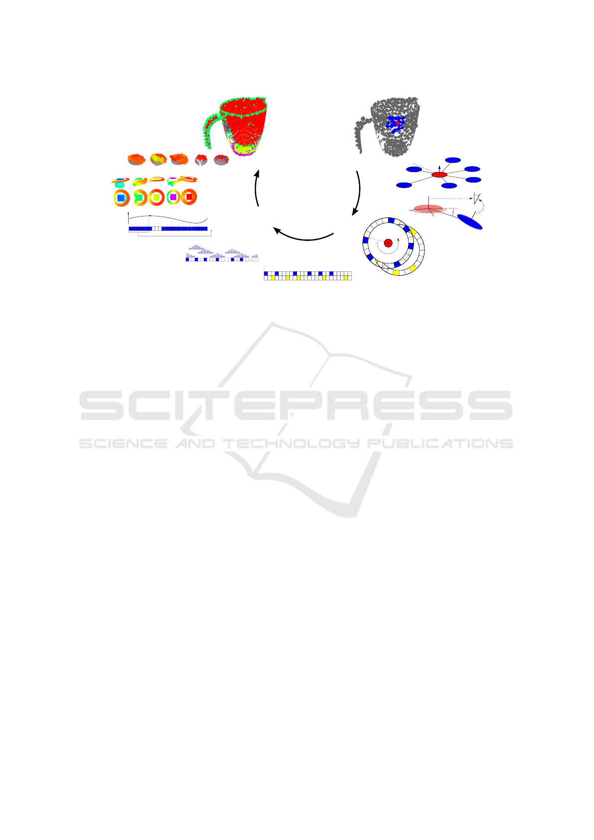
Figure 1: Overview of the feature creation and learning process for the SPGF feature. (a) A scene represented by τ features
with a selected one (red) and its neighbours (blue) within a radius, r. (b) Selected feature and its neighbours. (c) Spatial
relations between the central feature (red) and its neighbours. (d) Organization of the neighbours in two circular grid structures
introduced in the plane of the central feature, one grid describing features with the normal in the same direction as the central
one and one with normals pointing in the opposite direction of the central one. (e) Unfolding of the circular grids. (f)
Performing a weighted moving average filter to fill up empty cells in the grids. (g) Alignment of the grids to the direction
of highest curvature. (h) k-means clustering in the grid feature space resulting in a finite set of learned SPGF features. (i)
Features with associated grasp affordances. (j) Inferred features on object.
model based approaches where the unknown ob-
ject is approximated by simple shapes like bounding
boxes (e.g. (Curtis et al., 2008)) or more advanced
shapes like super-quadratics (e.g. (Huebner et al.,
2008)). Other model based approaches are for ex-
ample in (Detry et al., 2013) where object shapes are
learned as prototypical parts that human demonstrated
grasps are associated to. In work by (Kopicki et al.,
2014) a combined contact- and hand-model based on
visual appearance is learned for selecting successful
grasp poses.
The other main branch in vision based grasping
are feature based approaches, where visual features
are either used as cues or in a combined way used
as input for making grasp predictions. (Saxena et al.,
2008) showed how features from 2D images could
be used to find reliable grasp points for a dishwasher
emptying scenario. In work by (Kootstra et al., 2012),
it was shown how simple surface and edge features
could be used for predicting grasps with a reasonable
probability of success. In (Thomsen et al., 2015), vi-
sually triggered action affordances were learned by
associating related pairs of small surface patches with
successful grasping actions. Another feature-based
approach is proposed in work by (Lenz et al., 2013).
Here the visual feature representations were learned
unsupervised using deep learning techniques as a pre-
liminary step towards grasp learning. This work is of
particular interest as it showed superior performance
compared to a previous paper with fundamentally the
same grasp learning approach but where the visual
features were hand selected (Jiang et al., 2011). Other
approaches that utilise deep learning techniques for
unsupervised feature learning and later for grasp se-
lection are work by (Redmon and Angelova, 2014)
where AlexNet (Krizhevsky et al., 2012) has been
adopted to use RGB-D data as input. In work by (My-
ers et al., 2015), Superpixel Hierarchical Matching
Pursuit has been proposed and used to learn geomet-
ric visual features on RGB-D data on which tool af-
fordance learning has been applied. For an extensive
review of the work performed in the robotic grasping
domain see (J. Bohg and Kragic, 2014).
In our work, we propose a novel semi-local shape
descriptor, SPGF, aimed at grasp affordance learn-
ing. The SPGF feature allows for encoding of se-
mantically rich local surface structures, including
gaps and walls that can be found in multi-view or
SLAM (Durrant-Whyte and Bailey, 2006) acquired
scenes. When utilised for grasp affordance learn-
ing and prediction on previously unseen objects, the
learned features demonstrates high performance. As
the feature types are learned in an unsupervised
way using k-means clustering, they are not strictly
bound to the grasping actions and can therefore be
utilised for different actions although this utility is
only weakly exploited in this paper.
A Semi-local Surface Feature for Learning Successful Grasping Affordances
565
3 METHOD
The aim of the proposed SPGF feature is to provide
a solid foundation for reliable grasp affordance learn-
ing and prediction. To achieve this, a number of de-
sirable properties have been identified, that should be
captured by the feature:
1. Encoding of local shape geometry in SE(3).
2. Encoding of double sided structures.
3. Encoding of gaps.
4. Rotation invariance.
An overview of the process is shown in Fig. 1, where
the steps from object (Fig. 1a) to clustered reference
features (Fig. 1h), denoted prototypes, to grasp asso-
ciation (Fig. 1i) can be followed. In the following
subsections, first the feature creation process will be
explained (Fig. 1a–g and section 3.1), next the learn-
ing process of extracting a small finite set of descrip-
tive feature prototypes will be introduced (Fig. 1h and
section 3.2). In section 3.3, the feature inference pro-
cess, that allows for using the prototypes on novel sit-
uations will be addressed (Fig. 1j) and finally in sec-
tion 3.4, the learned features are linked to grasping
poses and grasp affordance learning (Fig. 1i).
As a starting point and input to the feature learning
system, a set of scenes, represented by small surface
patch descriptors (concretely texlets3D (Kraft et al.,
2014)) are used, see Fig. 1a for an example. As a
general notation the base features are described by a
position X and a surface normal vector n:
τ = {X, n} = {x, y, z, n
x
, n
y
, n
z
}, |n| = 1 (1)
3.1 Feature Creation
We start out with a scene representation consisting of
the above mentioned surfaces features (τ) and for each
surface feature we follow the steps sketched below:
1. Find all the neighbours, within an Euclidean ra-
dius r, see Figs. 1a, 1b. This leads to a context-
dependent number of neighbours (J).
2. For each of the J neighbours compute pairwise
spatial relations between the centre feature (red)
and the neighbour (blue). This will result in J pair-
wise relations, see Fig. 1c.
3. Split the neighbours into two sets based on the re-
lation of their normals with respect to the centre
feature; surface patches oriented in the same di-
rection make up one set of relations (r
t
), the others
the second (r
b
). Order the neighbours into two cir-
cular discretized grid structures based on the rota-
tion around the normal of the centre feature, see
Fig. 1d and Fig. 1e.
α
1
α
2
α
3
R
x
n
1
n
2
X
1
X
2
R
y
(a)
α
3
R
x
n
1
X
1
R
y
p(X
1
2
,R
y
)
p(X
1
2
,R
x
)
X
2
(b)
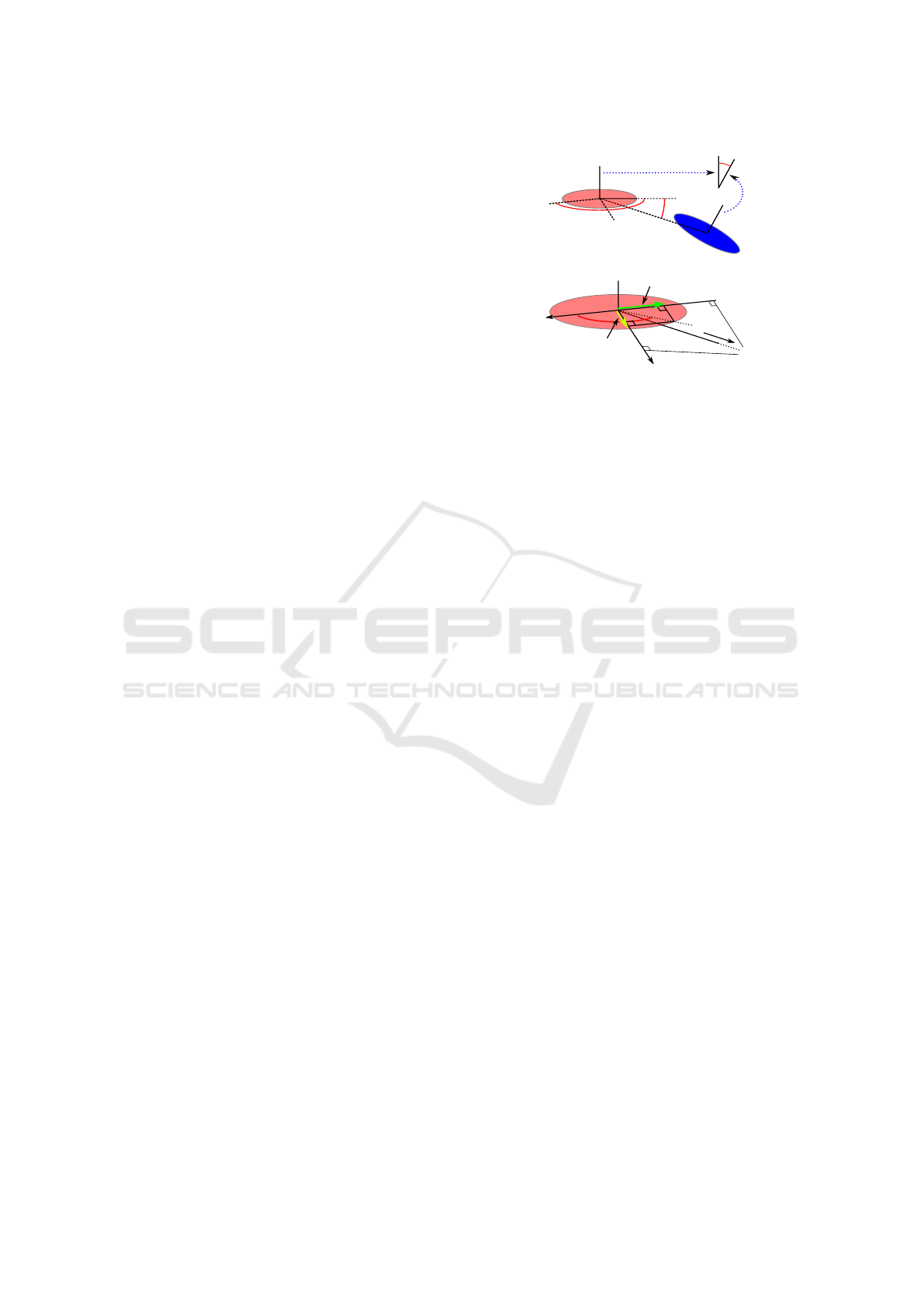
Figure 2: (a) The pairwise spatial relationships between the
centre feature (feature one) and feature two utilised in this
work. α
1
depict the angle between the plane of the cen-
tre feature (red) and the vector connecting the positions of
the features (X
2
1
), α
2
depicts the angle between the surface
normals of the two features, α
3
depicts the rotation angle
around the normal of the centre feature (n
1
) from a refer-
ence direction, R
x
, on the plane to the projection of the
connecting vector onto the plane. (b) A detailed view on
how the angle α
3
is derived from the projection of the vec-
tor X
2
1
onto the reference directions R
x
and R
y
(green and
yellow arrows), from which α
3
can be derived.
4. Fill out empty grid locations by applying a
weighted moving averaging filter over the grid
structures to combat sampling artefacts, see
Fig. 1f.
5. To achieve rotation invariance, the start point is
moved simultaneously for the two grids to the
grid-cell of highest curvature. In addition, the 6D
pose of the centre feature is corrected to align one
of the in plane axis with that direction, see Fig. 1g.
6. Finally, the top and bottom layer grids are con-
catenated into a feature vector, f , consisting of the
aligned 6D pose of the centre surface feature and
all the sorted relational values (r
0
t
,r
0
b
).
In the following subsections specific details are given
for the spatial relationships (step 2, section 3.1.1) and
the grid organizing (steps 3–6, section 3.1.2) proce-
dures.
3.1.1 Spatial Relationship
The relational descriptor used in this work is based
on a set of pairwise relations between surface patch
features of the type described in Eq. 1. The pairwise
relations resembles the ones proposed in (Wahl et al.,
2003) and (Mustafa et al., 2013). The three different
angular relations (α
1
, α
2
, α
3
) are visualised in Fig. 2
and described by Eqs. 2-4.
Before defining these angles a reference coordi-
nate system (R
x
, R
y
, n
1
) for the centre patch needs to
VISAPP 2016 - International Conference on Computer Vision Theory and Applications
566
Start
Start
α
3
Start
180
o
90
o
270
o
0
o
α
3
(a)
(b)
(c)
α
3
(d)
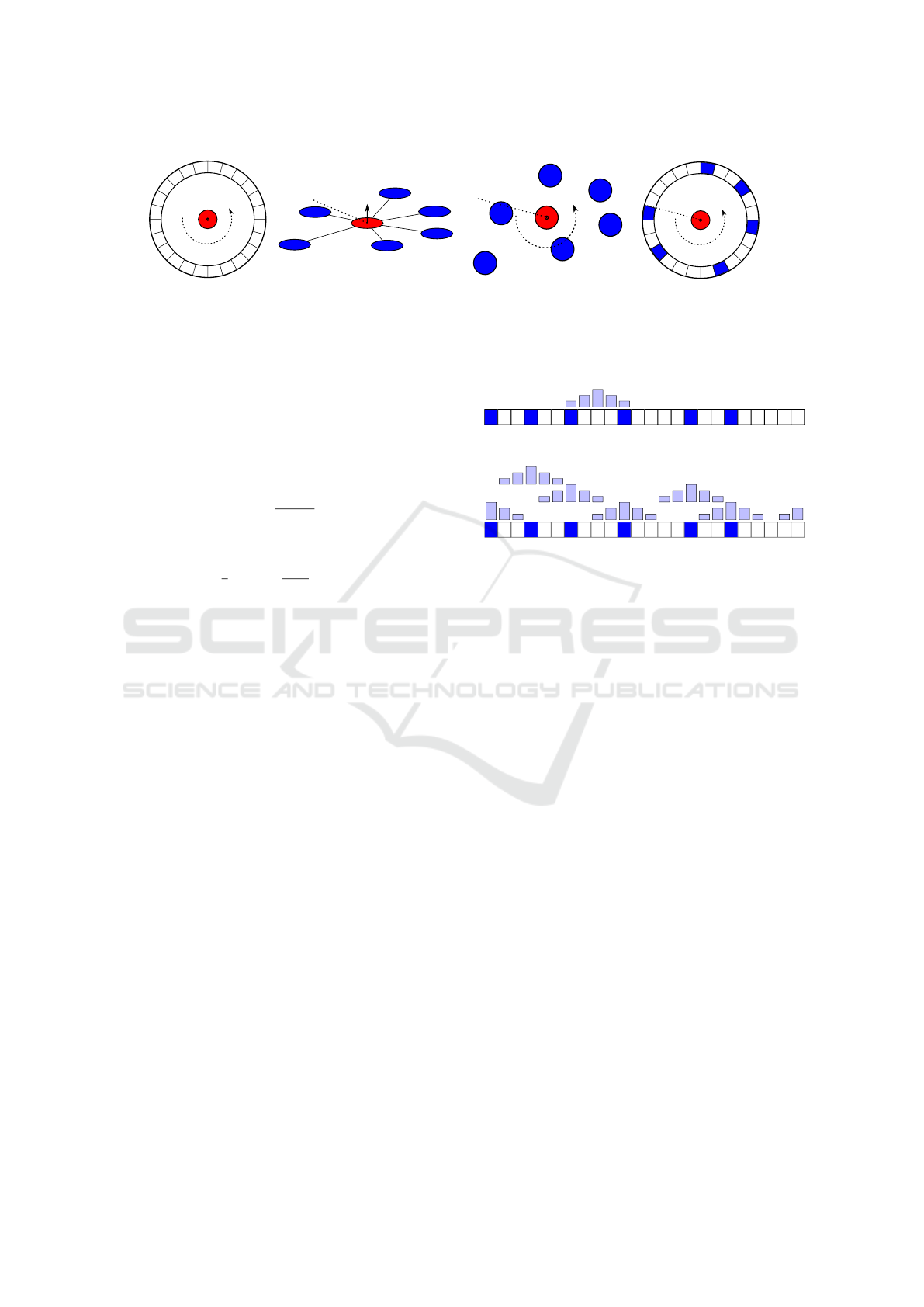
Figure 3: Introduction of the grid organization for a single layer (α
2
> 90
◦
or α
2
< 90
◦
). (a) The proposed grid structure
discretized into N
g
cells. (b) An example with six neighbours with an arbitrary start direction. (c) Top view of the projection
of the six neighbour positions in the plane of the red feature. (d) The six neighbours organised in the proposed discretized
grid structure based on their angle around the normal of the red feature, α
3
.
be defined. We choose the patch’s normal (n
1
) as z-
axis. R
x
is chosen to be an arbitrarily direction in the
plane of the first surface patch. The final axis (R
y
) can
then be computed using the cross product of n
1
and
R
x
. Furthermore the vector connecting the two fea-
tures (X
2
1
= X
1
−X
2
) and the projection of this vector
on an axis (p(X
2
1
, R
x
) =
(R
x
·X
2
1
)
||X
2
1
||
) are needed to then
define the angles between two features (τ
1
, τ
2
) as fol-
lows:
α
1
=
π
2
− acos(
X
2
1
||X
2
1
||
· n
1
) (2)
α
2
= acos(n
1
· n
2
) (3)
α
3
= atan2(p(X
2
1
, R
x
), p(X
2
1
, R
y
)) (4)
Together with the organisation in a grid structure, pre-
sented next, these measures are used to form the rela-
tional descriptor.
3.1.2 Organizing the Neighbourhood in a Sliced
Pineapple Grid Structure
The next step is to organize the information about
the neighbouring features into two circular grid struc-
tures. The two grid structures represent respectively
a top layer (r
t
) and a bottom layer (r
b
). The top layer
grid describes the neighbourhood of features with the
normal in the same direction (α
2
< 90
◦
) as the centre
feature and the bottom layer describes features with
the normal in the opposite direction of the centre fea-
ture (α
2
> 90
◦
).
Both layers are then discretized into a circular
grid, see Fig. 3(a), with a resolution of N
g
. All neigh-
bours are projected into the plane of the centre fea-
ture (see Fig. 3(c)) and their (α
1
, α
2
) are then placed
into the rotational bin that corresponds to the specific
α
3
value (see Fig. 3(d)). If multiple neighbours fall
within the same cell, the average value of the rela-
tions are used. These steps are performed for both, the
top layer and the bottom layer, resulting in two circu-
lar grids representing the neighbourhood of a feature.
The grids are then unfolded to two flat grids.
M
M+1
M+2
M-1
M-2
(a)
(b)
Figure 4: Weighted moving average of the grid structure.
(a) Illustrates how the cell at M is equally contributed to by
the cell at M+2 and M-2, practically resulting in the average
of the two. (b) A practical illustration of how the cells with
datapoints (coloured ones) affect the surrounding cells with
the weight depicted by the size of the bars.
Weighted Moving Average. Depending on the
number of neighbours within the radius, r, and the
discretization of the grid, the grid structures will con-
sist of a substantial amount of cells where no data is
found. These undefined cells are considered to be of
two types.
1. They are a result of the general low density of the
underlying feature representation within a small
radius.
2. They are real gaps depicting a direction where no
visual data exist.
The second type is of specific interest, as gaps can be
a strong visual cue (e.g., for affording pinch grasps or
indicating open structures), whereas the first type is
to be avoided. To address this artefact of sampling,
a weighted moving average (WMA) is performed on
the feature vectors to fill gaps. In addition, the WMA
improves the robustness of the feature representation.
In Fig. 4, the principle is illustrated by showing the
contribution that the existing datapoints give to neigh-
bouring cells in the grid, hereby filling out small gaps
in the representation. The WMA for the cells is per-
formed for the two relations (α
1
, α
2
) independently.
It should be noted, that if no value exists in a cell, it
A Semi-local Surface Feature for Learning Successful Grasping Affordances
567

will not contribute to the average. The length of the
filter n, determines the amount of smoothing.
After the moving average operation, gaps can still
exist depending on the length of the averaging filter.
These gaps are considered to be the “real” gaps. To
encode the real gaps in a meaningful way that can be
handled by the vector based k-means clustering, they
are described with saturated values of the parameters.
For α
1
this means −90
◦
and for α
2
this means 90
◦
and 180
◦
for the top and bottom grid respectively.
Alignment of Grid. As a final step, the feature grid
is aligned to make the representation rotation invari-
ant. The selected alignment is at the place of highest
curvature on the top part of the feature vector. This
equals finding the grid cell with the largest value of α
2
and reorganising the grid such that this cell becomes
starting point, see Fig. 5 and also Fig. 10, where the
alignment of the learned features are presented.
Start
Aligned
α
2
α
2
,max
Reorganize grid
Figure 5: Alignment of the feature grid starting point based
on the maximum value of α
2
, α
2,max
, of the top layer grid.
The variation of α
2
over the grid is visualised above the
grid. Both top layer and bottom layer are aligned to this new
starting point and the grids are reorganized accordingly.
Based on the aligned starting point, a 6D pose is
computed (update the reference direction R
x
and R
y
,
see subsection 3.1.1) to place the feature with respect
to the world. Finally, the aligned top (r
0
t
) and bottom
(r
0
b
) grids are concatenated into a combined feature
vector f and the aligned 6D pose of the centre feature
is added.
3.2 Feature Learning
Once this representation is designed, we are interested
in finding reference features, called prototypes, that
are able to describe the features present in the training
object scenes in the best way. For that the following
two steps are taken.
1. Perform the feature creation steps, see section 3.1,
for the full object set, resulting in a large set of
feature vectors, f
i
: i = 1, ..., L
2. Perform a k-means Euclidean clustering (Lloyd,
2006) in the relational space of the f ’s (only the
r
0
t
, r
0
b
parts, not the position or orientation of the
centre). K defines the number of prototypes (P
id
)
that the learned dictionary, (P) Eq. 6, should con-
sist of. The prototypes are described by a point in
the relational-vector space, see Eq. 5 and Fig. 1h.
P
id
= {α
0
1,id
, α
0
2,id
, α
1
1,id
, α
1
2,id
, ...,
α
2N
g
−1
1,id
, α
2N
g
−1
2,id
} ∈ R
2·2N
g
(5)
P = {P
1
, P
2
, ..., P
K
} (6)
3.3 Feature Inference
Provided a set of feature prototypes has been learned,
the inference process of utilising them to describe
novel objects is introduced with the following steps:
1. Perform the feature creation process, see sec-
tion 3.1, for an object where features are to be
inferred. This results in a set of feature vectors
F.
2. For every f ∈ F, find the closest prototypes P
id
in the set of learned prototypes P using the Eu-
clidean distance on the relation part (only r
0
t
, r
0
b
)
of f , see Eq. 7. Given this id, a new feature T is
created that consists of the feature pose (position
X and quaternion q ,given by f ) and the computed
id. See also Fig. 1j for an example object with in-
ferred features.
D( f , P
id
) =
v
u
u
t
2N
g
−1
∑
i=0
(α
i
1, f
− α
i
1,id
)
2
+ (α
i
2, f
− α
i
2,id
)
2
(7)
id = argmin
id
(D( f , P
id
) : P
id
∈ P) (8)
T = {X, q, id} (9)
3.4 Grasp Affordance Learning
In order to utilize the learned SPGF features for grasp
affordance learning (Fig. 1i), the pose of the visual
feature is linked to the pose of a grasp by a 6D pose
transformation, see Fig. 6. We use the method intro-
duced by (Thomsen et al., 2015) to do this. In the
following, we give a brief overview of the method for
details please see (Thomsen et al., 2015).
The shape-grasp space is occupied by a large set
of shape-grasp particles describing how individual ac-
tions relate to individual features. To condense the
information for reliable action predictions, a neigh-
bourhood analysis is performed to compute the suc-
cess probability of a given point in the space as well
as the amount of similar points (called support). Next,
the learned shape-grasp particle space is condensed
to only consist of points that have a significant sup-
port. This knowledge is then used to vote for grasps
VISAPP 2016 - International Conference on Computer Vision Theory and Applications
568
in novel situations with the probability associated dur-
ing learning. This results in a set of grasps, that can
be ranked based on the predicted success probability
and the amount of votes.
4 EXPERIMENTS
The experiments performed in this work are
based on a simulated set-up created in RobWork-
Sim (Jørgensen et al., 2010), see Fig. 7. The set-up
consists of simulated RGB-D sensors and the object
of interest in the centre, from which a visual object
representation is acquired, see Fig. 7a and Fig. 1a for
an extracted scene. It should be noted that modelled
sensor noise is added and that the four views still lead
to incomplete models that the four views introduce. In
addition to the scene rendering, the simulation envi-
ronment is also utilised for performing grasping sim-
ulations by means of the simulation framework Rob-
WorkSim. The simulator is based on a dynamics en-
gine that simulates object dynamics in terms of the
contact forces that emerge during a grasping execu-
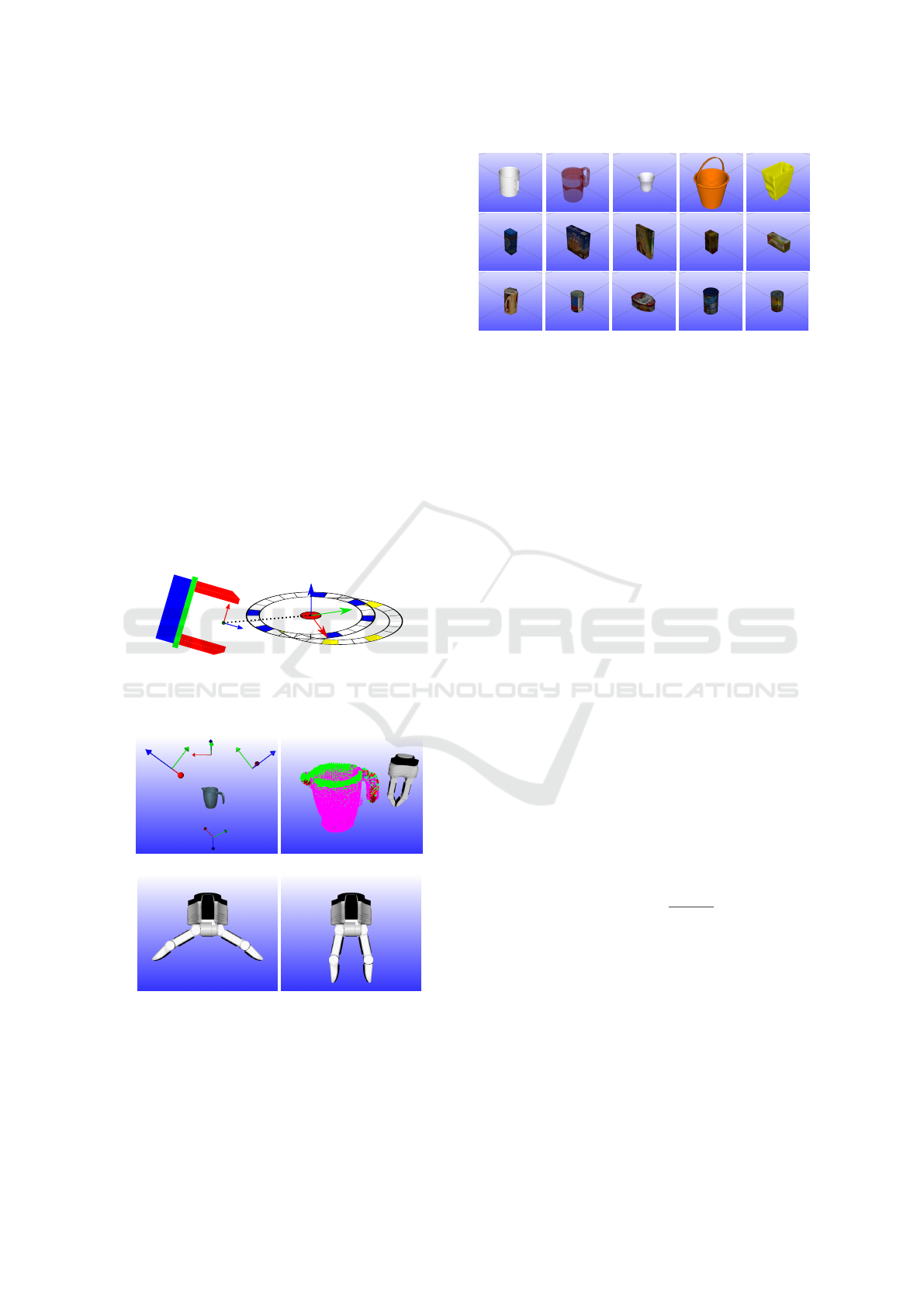
Start
0
o
α
3
T
Figure 6: Linking of a grasping action and a visual fea-
ture, T, described by the 6D pose transformation, a grasp
outcome (success/failure) and an id (relating to the corre-
sponding P
id
).
(a) (b)
(c) (d)
Figure 7: Experimental setup. (a) Visualisation of the sim-
ulated sensor set-up. Four RGB-D sensors, represented by
the four frames, surround the object. (b) Outcome of grasp
simulations performed in RobWorkSim (Jørgensen et al.,
2010) with the NPG (Narrow Pinch Grasp), see (d). Red
and pink equals failed grasps and green depicts successful
grasps. (c) The Wide Pinch Grasp (WPG).
Figure 8: A subset of the 50 objects used in the ex-
perimental work. The 3D models have been taken
from the KIT database (Kasper et al., 2012) and from
archive3d (Archive3D, ). See (Thomsen et al., 2015) for
the full object set.
tion. Grasping is performed with a simulated version
of the Schunk SDH-2 hand with two different grasp
preshapes, a wide pinch grasp (WPG) and a narrow
pinch grasp (NPG), see Figs. 7(c) and 7(d). The ex-
periments are performed on an object set consisting of
50 objects, see Fig. 8 for a subset. The object are clas-
sified into three classes, containers, boxes and curved
objects.
Evaluation Score. A 5-fold cross-validation is per-
formed to evaluate the learned prototypes for predic-
tion of grasps on novel objects. The learning and eval-
uation of features and grasps are performed on the full
object set. However, in order to compare the achieved
results with work of (Thomsen et al., 2015) on the
same dataset the object class-wise grasp prediction
performance is also presented.
To measure the performance of our method, we
use the success-rate of the highest ranked grasps from
the votes of shape-grasp particles. The N highest
ranked grasps (in a combined selection of support and
probability, here the support depict that a grasp have
achieved a significant amount of votes) are compared
to the actual outcome of the grasps and the success-
rate is computed as follows:
success-rate =
N
success
N
(10)
Feature Learning Parameters. For the feature
learning part five parameters need to be set. A radius,
r, of 0.03m is used. The discretization of the circu-
lar grid, N
g
, is set to 36, equalling slices of 10
◦
. The
WMA filter is set to be of length 6 resulting in an av-
erage over 60
◦
in each direction. Finally, the amount
of clusters, (K learned features), are varied between
5 and 25 as a part of the experimental results. In the
presented results N=10 is used.
.
A Semi-local Surface Feature for Learning Successful Grasping Affordances
569
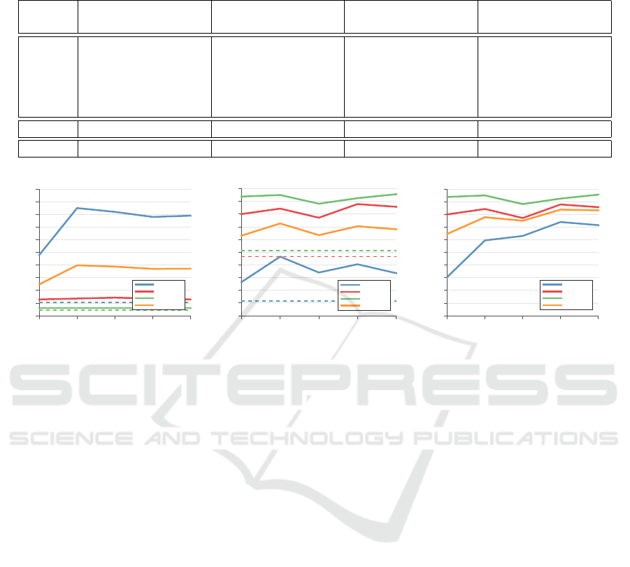
Table 1: Success-rate for Narrow Pinch Grasp (NPG), Wide Pinch Grasp (WPG) and Combined Grasp (CG). Results are
based on the average success-rate of the 10 highest predicted grasps for each object. Random depict the chance for randomly
selecting a successful grasp in the set. [*] depict the results achieved in (Thomsen et al., 2015).
Containers [%] Boxes [%] Curved [%] All [%]
NPG WPG CG NPG WPG CG NPG WPG CG NPG WPG CG
K
5 48.0 26.5 30.5 12.9 80.0 80.0 6.3 93.8 93.8 24.8 63.0 64.6
10 85.0 46.5 59.5 13.6 84.3 84.3 6.3 95.0 95.0 39.8 72.6 77.8
15 82.0 34.0 63.0 14.3 77.1 77.1 6.3 88.1 88.1 38.8 63.4 75.0
20 78.0 40.5 74.0 13.6 87.9 87.9 6.3 92.5 92.5 37.0 70.4 83.8
25 79.0 33.5 71.5 12.9 85.7 85.7 6.3 95.6 95.6 37.2 68.0 83.2
[*] 68 - - - 84 - - 84 - - - -
random 10.6 11.5 - 4.8 46.6 - 4.4 51.3 - 7.0 34.1 -
Number of features (K)
5 10 15 20 25
Success-rate
0
0.1
0.2
0.3
0.4
0.5
0.6
0.7
0.8
0.9
1
NPG
Containers
Boxes
Curved
All
Number of features (K)
5 10 15 20 25
Success-rate
0
0.1
0.2
0.3
0.4
0.5
0.6
0.7
0.8
0.9
1
WPG
Containers
Boxes
Curved
All
Number of features (K)
5 10 15 20 25
Success-rate
0
0.1
0.2
0.3
0.4
0.5
0.6
0.7
0.8
0.9
1
CG
Containers
Boxes
Curved
All
Figure 9: The results for the grasp predictions for the different object classes as well as for all the objects, presented for the
two different grasp types NPG and WPG and for the combined grasp CG. The dashed lines depict the random chance of
selecting a successful grasp for the individual object classes.
5 RESULTS
First, an evaluation of the grasp prediction perfor-
mance is presented for different amounts of learned
features (different K’s) (section 5.1). Secondly, a
qualitative assessment of a set of learned features and
learned associated grasps is presented (section 5.2).
5.1 Grasp Prediction Evaluation
In Tab. 1 and Fig. 9, the results are presented for the
individual object classes for the two different grasp
types (NPG, WPG) (see Fig. 7) as well as for the grasp
performance when the highest ranked of the two grasp
types are chosen (CG). These measures are also pre-
sented for the full object set. All the results are pre-
sented for five different values of K. The table also
shows the performance in (Thomsen et al., 2015) and
the chance for a random selected grasp to be success-
ful.
For the container objects, the performance of the
NPG grasp is generally high around 80% for K larger
than five, whereas the performance with WPG grasp
is in the range of 27% – 47%. When the best of the
two grasp types is chosen, CG, the performance is in
the range of 60% – 74% for K larger than five. The
scores should be compared with the random chance
of selecting one of the two grasps (11%). For the box
objects, the NPG grasp have a success-rate in the re-
gion of 10% – 15% whereas the WPG grasp performs
with a success-rate in the range of 77% – 88%. Sim-
ilar results as the WPG is achieved for the CG grasp.
For the curved objects, the NPG grasp have a success-
rate of 6% and the WPG grasp performs in the range
of 88% – 95%. The CG grasp performs similar to the
WPG grasp. For all the objects, the NPG grasp per-
formance is in the range of 25% – 40% whereas the
WPG performs in the range of 63% – 73%. When
combined, the performance goes up to be in the range
of 65% – 84%.
When comparing the scores for the individual
grasp types, NPG and WPG, with the performance of
the CG, we see, that for the container objects the CG
score (31% – 74%) is performing worse than the NPG
(48% – 85%) and the WPG (27% – 41%) whereas
for the Box and Curved objects the CG performance
(77% – 87% and 88% – 96%) is comparable to the
score of the highest of the individual grasp types (88%
and 95%). This difference is explained by the fact
that the random chance of selecting a successful WPG
VISAPP 2016 - International Conference on Computer Vision Theory and Applications
570
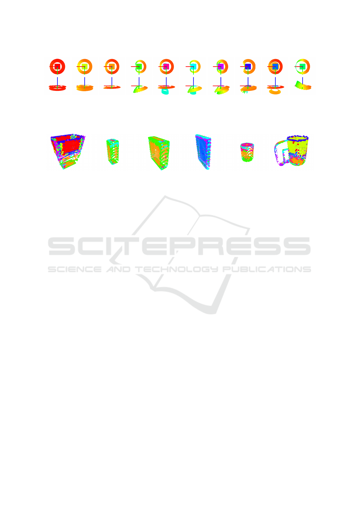
Figure 10: Visualisation of a learned set of visual features with K=10. The features are denoted 1 to 10 from left to right.
The bottom and top rows show the same features from different angles. In addition to the actual inclination of the outer ring
feature, the colour also denote the angle difference to the normal of the centre feature, green/cyan depict strong curvature
whereas red depict none or little curvature. The orientation of the features are described by the inlaid frames (red, green and
blue sticks). The colour in the centre of the features is used for encoding the inferred features on the novel objects, see Fig. 11.
Figure 11: Example objects with inferred learned features. See the features in Fig. 10 and the corresponding colour coding to
interpret the objects.
grasp is significantly higher than the chance for ran-
domly selecting a NPG grasp. For the container ob-
ject set it means that the grasp votes from the WPG
learned affordances tend to dominate the NPG learned
affordances, resulting in the lower combined score.
When comparing the results with the achieved
scores in (Thomsen et al., 2015), superior perfor-
mance is achieved, despite the fact that the conditions
for the results acquired in this work is significantly
more difficult due to that visual and action training
is performed on the full object set as compared to
the class-wise approach in (Thomsen et al., 2015).
The performance on the individual object classes for
the NPG and WPG perform better than the results
acquired in (Thomsen et al., 2015) for the largest
amount of Ks and in particular for K larger than five.
The CG performance for the different classes also per-
forms better than the individual grasps from (Thom-
sen et al., 2015) for a specific K. For K=20, the CG
container score (74%) outperforms the NPG score
(68%) from (Thomsen et al., 2015). For the boxes, the
CG score (87%) outperforms the WGP score (84%)
from (Thomsen et al., 2015) and for the curved ob-
jects, the CG score (93%) outperforms the WPG score
(84%) from (Thomsen et al., 2015). Finally, the
achieved score of 84% probability for selecting a suc-
cessful grasp, CG, for the full object set is compara-
ble to the highest achieved score for the individually
grasp types in (Thomsen et al., 2015) for K=20.
5.2 Qualitative Assessment
In Fig. 10, the learned features from one of the folds
are visualised for K=10. In Fig. 11, a subset of the
novel objects in the same fold is shown with inferred
features. The second figure can be useful to under-
stand what the features describe. Multiple meaningful
structures can be identified when assessing the fea-
tures qualitatively, see Fig. 10. There are wall fea-
tures with different curvature (1 and 2). Walls at an
edge (7). Wall that have a gap which is identified as
a rim (8). A surface feature with slight curvature (3)
and surface edge structures (4, 5 and 6) with a varying
degree of curvature.
In Figs. 12 and 13, the learned visual features are
shown with the associated learned grasp affordances,
in terms of coloured stick figures that depict the orien-
tation of the grasps with respect to the feature. When
assessing the features from the NPG (Fig. 12), only
feature eight seems to be a reliable predictor for suc-
cessful grasps. This feature describes the rim of a wall
which explains the good performance as it intuitively
is a good place to try a narrow pinch grasp. Some of
the other features show some performance potential,
for instance feature one, that describes a wall struc-
ture. A wall is intuitively graspable by a NPG grasp,
but because it is found in a uniform area, one DOF
in the pose is ill defined resulting in a low but rather
uniform success probability around this DOF.
For the case of the WPG grasp, visualised in
Fig. 13, the results are quite different. For the mostly
flat structures (1 and 3), areas of high probability are
not found. However for the highly curved features
that somehow relate to edges (2, 4, 6 and 10) there are
structures that suggest very high likelihood of grasp
success. For features (2, 4 and 10) high probability
areas are found in a somehow box structure aligned to
the feature and below the features (the third column
shows the bottom view). For feature six, the high
probability areas are also found towards the normal
A Semi-local Surface Feature for Learning Successful Grasping Affordances
571
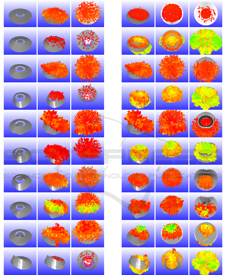
Figure 12: Visualisation of the visual features with the
learned grasp affordances for the NPG grasp. The features
are denoted 1 to 10 from top to bottom. Red depict low
probability (0.0) of success. The colour changes towards
green that depict a success probability of 1.0. First column
show the features, the second column show the features with
associated grasp from a perspective view and the third col-
umn show the features from a top view.
Figure 13: Visualisation of the visual features with the
learned grasp affordances for the WPG grasp. The features
are denoted 1 to 10 from top to bottom. Red depict low
probability (0.0) of success. The colour changes towards
green that depict a success probability of 1.0. First column
shows the features from a perspective view. The second col-
umn, from a top view and the third column, from a bottom
view. See also the first column of Fig. 12 for a view of the
features without grasps.
VISAPP 2016 - International Conference on Computer Vision Theory and Applications
572

of the centre feature. When this is matched with the
inferred features on the fourth object in Fig. 11, this
seems reasonable.
Finally, the qualitative result show that a diverse
set of features are needed for predicting even slightly
different actions with high rates of success. Exempli-
fied by the fact that only a single prototype is good
for the NPG grasp whereas others are suitable for the
WPG grasp. This is an indication that our unsuper-
vised approach for prototype learning based on the
occurrence in the object set is a reasonable way to go.
6 CONCLUSION
In this paper, we have proposed, the Sliced Pineapple
Grid Feature (SPGF), a novel semi-local shape-based
descriptor, with the aim of utilising it for grasp affor-
dance learning. The descriptor has a number of key
properties such as its ability to encode double sided
structures, encoding of gaps as well as being rota-
tional invariant. As the extraction of a specific dis-
crete set of shape descriptors is based on an unsuper-
vised approach, the amount of features can be tuned
for different applications or object sets. When utilis-
ing the learned features for grasp affordance learning
and afterwards use the learned knowledge on novel
situations, our system is able to predict grasp success
with a rate of up to 96% for individual object classes
and up to 84% when applied to an object set consist-
ing of three classes of objects.
By utilising the learned features, the performance
is better or comparable to the best results achieved in
(Thomsen et al., 2015) performed on the same dataset
despite that the learning conditions in this work are
significantly more difficult. Regardless of the re-
spectable performance of the grasp affordance system
when applied to the full object set, the potential of the
system is not yet fully realized, primarily illustrated
by the fact that the CG performance for the container
objects is well below the highest achieved score for
the individual grasp types WPG and NPG. The pri-
mary reason for this is an unbalanced dataset, as the
chance of randomly selecting a successful WPG grasp
is significantly higher than the chance of randomly se-
lecting a NPG grasp. This means that the votes from
WPG tend to dominate the votes from NPG, resulting
in a worse combined score.
From a qualitative perspective, the learned fea-
tures exhibit similarity to structures that can be iden-
tified as building blocks of objects such as “walls”,
“rims”, “edges”, “surfaces” and others. Furthermore,
the results indicate that different features are suitable
for different affordances, in our work demonstrated
by the two grasp types. Given the intuitiveness of the
learned surface structure, a natural next step is to com-
bine these into more elaborated features.
ACKNOWLEDGEMENT
The research leading to these results has received
funding from the European Community’s Seventh
Framework Programme FP7/2007-2013 (Specific
Programme Cooperation, Theme 3, Information and
Communication Technologies) under grant agree-
ment no. 270273, Xperience.
REFERENCES
Archive3D. Archive3d free online cad model database.
http://www.archive3d.net.
Curtis, N., Xiao, J., and Member, S. (2008). Efficient
and effective grasping of novel objects through learn-
ing and adapting a knowledge base. In IEEE In-
ternational Conference on Robotics and Automation
(ICRA), pages 2252–2257.
Detry, R., Ek, C. H., Madry, M., and Kragic, D. (2013).
Learning a dictionary of prototypical grasp-predicting
parts from grasping experience. In IEEE International
Conference on Robotics and Automation.
Durrant-Whyte, H. and Bailey, T. (2006). Simultaneous lo-
calization and mapping: part i. Robotics Automation
Magazine, IEEE, 13(2):99–110.
Huebner, K., Ruthotto, S., and Kragic, D. (2008). Mini-
mum volume bounding box decomposition for shape
approximation in robot grasping. In Robotics and Au-
tomation, 2008. ICRA 2008. IEEE International Con-
ference on, pages 1628–1633. IEEE.
J. Bohg, A. Morales, T. A. and Kragic, D. (2014). Data-
driven grasp synthesis a survey. IEEE Transactions
on Robotics, 30(2):289–309.
Jiang, Y., Moseson, S., and Saxena, A. (2011). Efficient
grasping from rgbd images: Learning using a new
rectangle representation. In ICRA’11, pages 3304–
3311.
Jørgensen, J. A., Ellekilde, L.-P., and Petersen, H. G.
(2010). RobWorkSim - an Open Simulator for Sensor
based Grasping. Robotics (ISR), 2010 41st Interna-
tional Symposium on and 2010 6th German Confer-
ence on Robotics (ROBOTIK), pages 1 –8.
Kasper, A., Xue, Z., and Dillmann, R. (2012). The KIT
object models database: An object model database
for object recognition, localization and manipulation
in service robotics. The International Journal of
Robotics Research.
Kootstra, G., Popovi
´
c, M., Jørgensen, J. A., Kuklinski, K.,
Miatliuk, K., Kragic, D., and Kr
¨
uger, N. (2012). En-
abling grasping of unknown objects through a syner-
gistic use of edge and surface information. Has been
accepted for Internation Journal of Robotic Research.
A Semi-local Surface Feature for Learning Successful Grasping Affordances
573

Kopicki, M., Detry, R., Schmidt, F., Borst, C., Stolkin, R.,
and Wyatt, J. L. (2014). Learning dexterous grasps
that generalise to novel objects by combining hand
and contact models. In to appear in IEEE Interna-
tional Conference on Robotics and Automation.
Kraft, D., Mustafa, W., Popovic, M., Jessen, J. B., Buch,
A. G., Savarimuthu, T. R., Pugeault, N., and Kr
¨
uger,
N. (2014). Using surfaces and surface relations in an
early cognitive vision system. Computer Vision and
Image Understanding.
Krizhevsky, A., Sutskever, I., and Hinton, G. E. (2012). Im-
agenet classification with deep convolutional neural
networks. In Advances in neural information process-
ing systems, pages 1097–1105.
Kr
¨
uger, N., Janssen, P., Kalkan, S., Lappe, M., Leonardis,
A., Piater, J., , Rodr
´
ıguez-S
´
anchez, A. J., and Wiskott,
L. (2013). Deep hierarchies in the primate visual cor-
tex: What can we learn for computer vision? IEEE
PAMI, 35(8):1847–1871.
Lenz, I., Lee, H., and Saxena, A. (2013). Deep learning for
detecting robotic grasps. CoRR , pages –1–1.
Lloyd, S. (2006). Least squares quantization in pcm. IEEE
Trans. Inf. Theor., 28(2):129–137.
Mustafa, W., Pugeault, N., and Kr
¨
uger, N. (2013). Multi-
view object recognition using view-point invariant
shape relations and appearance information. In IEEE
International Conference on Robotics and Automation
(ICRA).
Myers, A., Teo, C. L., Ferm
¨
uller, C., and Aloimonos, Y.
(2015). Affordance detection of tool parts from geo-
metric features. In ICRA.
Redmon, J. and Angelova, A. (2014). Real-time grasp de-
tection using convolutional neural networks. CoRR,
abs/1412.3128.
Saxena, A., Driemeyer, J., and Ng, A. Y. (2008). Robotic
grasping of novel objects using vision. Int. J. Rob.
Res., 27:157–173.
Thomsen, M., Kraft, D., and Kr
¨
uger, N. (2015). Identi-
fying relevant feature-action associations for grasping
unmodelled objects. Paladyn, Journal of Behavioral
Robotics.
Wahl, E., Hillenbrand, U., and Hirzinger, G. (2003). Surflet-
pair-relation histograms: a statistical 3d-shape repre-
sentation for rapid classification. In 3-D Digital Imag-
ing and Modeling, 2003. 3DIM 2003. Proceedings.
Fourth International Conference on, pages 474–481.
IEEE.
VISAPP 2016 - International Conference on Computer Vision Theory and Applications
574
