Feature-augmented Trained Models for 6DOF Object Recognition and
Camera Calibration
Kripasindhu Sarkar
1,2
, Alain Pagani
1
and Didier Stricker
1,2
1
German Research Center for Artificial Intelligence (DFKI), Kaiserslautern, Germany
2
Technical University Kaiserslautern, Kaiserslautern, Germany
Keywords:
6DOF Object Recognition, Calibration, Natural Calibration Rigs, Feature-augmented 3D Models.
Abstract:
In this paper we address the problem in the offline stage of 3D modelling in feature based object recognition.
While the online stage of recognition - feature matching and pose estimation, has been refined several times
over the past decade incorporating filters and heuristics for robust and scalable recognition, the offline stage of
creating feature based models remained unchanged. In this work we take advantage of the easily available 3D
scanners and 3D model databases, and use them as our source of input for 3D CAD models of real objects. We
process on the CAD models to produce feature-augmented trained models which can be used by any online
recognition stage of object recognition. These trained models can also be directly used as a calibration rig for
performing camera calibration from a single image. The evaluation shows that our fully automatically created
feature-augmented trained models perform better in terms of recognition recall over the baseline - which is
the tedious manual way of creating feature models. When used as a calibration rig, our feature augmented
models achieve comparable accuracy with the popular camera-calibration techniques thereby making them an
easy and quick way of performing camera calibration.
1 INTRODUCTION
The progress in the field of Structure From Motion
(SFM) made it possible to have 3D models recon-
structed from unordered images. Since these models
are a result of matching features across several im-
ages, any 3D point in the reconstructed sparse model
can be associated with a variety of view dependent de-
scriptors. This association of 3D points - to - 2D de-
scriptors forms the pillar of most of the feature based
detection where the features, extracted from a given
input image, are matched to that of the feature aug-
mented 3D models and subsequently, a 6 DOF recog-
nition is made [Skrypnyk and Lowe, 2004, Hao et al.,
2013, Collet Romea et al., 2011, Collet Romea and
Srinivasa, 2010, Irschara et al., 2009].
Therefore, we can summarize all the feature based
recognition methods in the following steps:
1. Building models (offline training stage). In the
first step, feature-augmented-3D-models are con-
structed for each of the objects which is to be
recognized. For each of the real objects, a set
of images from several directions are taken (usu-
ally around 50 - 80 [Collet Romea and Srinivasa,
2010, Collet Romea et al., 2011]), SFM is per-
3D CAD Models
6DOF Recognition
Learning Feature-
Augmented
Model
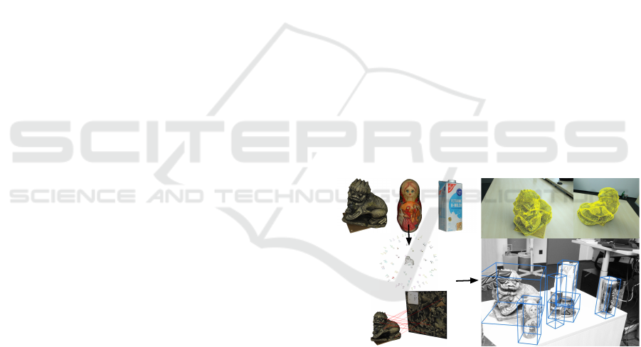
Figure 1: Feature-augmented models for 6DOF object
recognition. Starting with 3D CAD models our method
produces ‘trained-models’ that can be used by any online
recognition framework for 6DOF recognition.
formed, and then finally, view dependent features
for each 3D point in the obtained reconstruction
are merged using a clustering or averaging tech-
nique. In the end of this step we have a set of
feature-augmented-3D-models which we will re-
fer here as ’model’.
2. Recognition (online stage). The online stage in-
volves object recognition in a query image using
the models learnt in the offline stage. Image fea-
tures extracted from the query image are matched
632
Sarkar, K., Pagani, A. and Stricker, D.
Feature-augmented Trained Models for 6DOF Object Recognition and Camera Calibration.
DOI: 10.5220/0005781106320640
In Proceedings of the 11th Joint Conference on Computer Vision, Imaging and Computer Graphics Theory and Applications (VISIGRAPP 2016) - Volume 4: VISAPP, pages 632-640
ISBN: 978-989-758-175-5
Copyright
c
 2016 by SCITEPRESS – Science and Technology Publications, Lda. All rights reserved

against those in the stored models to get sets of
2D-3D correspondences. Using the correspon-
dences, the pose of the object is found by solving
for the projection matrix by one of the dedicated
Perspective-n-Points (PnP) methods [Dementhon
and Davis, 1995,Lepetit et al., 2009]. This step is
usually integrated with outlier removal methods to
handle outliers introduced in the matching stage.
There has been several variations of the online
stage [Skrypnyk and Lowe, 2004,Collet Romea et al.,
2011, Hao et al., 2013] - mostly to make the recogni-
tion faster and robust, but the training stage remained
more or less unaltered in its original form. The in-
herent problem in the offline training stage is unad-
dressed in all the available methods. The problem lies
in the amount of manual work involved to create a
feature-augmented-3D-model. The main pain-point is
to take hundreds of pictures for each model and seg-
ment each of them manually before feeding them to
SFM. [Hao et al., 2013] used a painted turntable top
and a clean background with controlled lighting to re-
duce the pain of manual capturing, but it still produces
lot of outlier model points. Also, producing models
on such a controlled environment for object recogni-
tion is not scalable to new objects in a new location.
In this paper we address the problem associated
with the training stage and propose a method to elim-
inate all the manual work involved in the existing
methods. Here, we accept 3D CAD models to be
recognized as input, and produce trained feature-
augmented-models as output which can be used by
the online stages of any of the recognition methods
stated above.
Since the information of 3D to 2D correspon-
dences is already available and encoded in our trained
model, we can directly leverage this information to
find the intrinsic of the query image. Therefore, we
provide a way of directly calibrating an image con-
taining one of the models. Our models trained out
of ordinary objects can be just used as a marker for
performing calibration without the need of specially
designed calibration rigs.
Therefore, our contribution for this paper is a set
of algorithms and methods which operates on 3D
CAD models to produce feature augmented models
for 6DOF recognition and calibration. Because of the
capability of the trained models for performing recog-
nition with full pose, our method is very practical for
robotic manipulations of objects (such as grasping or
other interactions) starting from a single 2D image
frame.
It might appear that acquiring CAD models for it-
self can be a tedious task. But, this is not true in the
present situation where cheap and accurate 3D scan-
ners are available in most Robotics and Vision labs.
This is because of the boost in a separate branch of re-
search in the topic of 3D computer vision and object
recognition/registration in 3D point clouds. In many
of these methods, CAD models remain the source
of input for processing and extracting different fea-
tures or other information which are used with that of
the scene point-cloud for solving a particular problem
(eg. 3D recognition) [Tombari et al., 2010,Rusu et al.,
2010, Aldoma et al., 2012]. We do a similar task and
process on CAD models to extract information. But
instead of point cloud, we perform a full 6DOF recog-
nition in a simple 2D image using the processed data.
Our approach can be viewed as the combination of
techniques from 2D and 3D computer vision.
In addition to the large variety of easily available
3D scanning hardwares [D’Apuzzo, 2006], we also
have now simple software solutions for 3D acquisi-
tion where CAD models can be acquired using off-
the-shelf hardware. The scanner we used in our ex-
perimentation, 3Digify [3Digify, 2015], is one such
example where any two household cameras and a pro-
jector can be used with the software to make a power-
ful 3D scanner.
Our methods use two ways to generate 3D points
- 2D features correspondences. The first approach is
a simple method that uses the texture maps associ-
ated with the 3D models to get the 2D feature in-
formation for 3D points. The second approach is
more closer to the traditional method that takes vir-
tual snapshots of the 3D model from several direc-
tions based on a snapshot model and subsequently
matching features among the snapshots to rebuilt a
feature-augmented model. Our methods along with
the recognition pipeline is summarized in Figure 1.
The details of the methods are provided in the Sec-
tion 3.
2 RELATED WORK
Object recognition is one of the key topic in Computer
Vision involving several techniques. In this section
we will limit our focus to 6DOF object recognition
methods which uses 2D local features. This has been
a very popular topic which started with the invention
of the robust local feature descriptors - SIFT [Lowe,
2004]. The first application of these descriptors to-
wards pose detection in a scene, used them to com-
pute multi-view matches and perform structure from
motion to generate feature-augmented scene model.
This learned model was then used for scene recogni-
tion with full pose estimation [Skrypnyk and Lowe,
2004].
Feature-augmented Trained Models for 6DOF Object Recognition and Camera Calibration
633

The most robust recognition application in this
principle is MOPED [Collet Romea et al., 2011]
where the authors perform the online recognition
stage efficiently by clustering the features in the im-
age space before searching for an object, removing
many outliers in this process before the matching step.
Their training stage still uses the same technique of
taking multiple images (around 50) of objects from
different directions, segment them manually and then
feed them to their training software. Even with their
elegant online recognition technique, adding training
models to be recognized still becomes problematic
and inconvenient because of the amount of manual
work involved in the training stage.
The latest work in this area is [Hao et al., 2013]
which once again address the problems in the online
stage to make it more scalable and robust. To handle
spurious 2D-to-3D correspondence that increases the
number of RANSAC iterations, the authors proposed
efficient filtering methods in the first place. They ap-
plied a local filtering step which efficiently checks ev-
ery individual correspondence in a local region, based
on both statistical and geometric cues including spa-
tial consistency and co-visibility. They further filter
the spurious correspondences by a global filtering step
which is performed on every correspondence pairs
which leverage some finer-grained 3D geometric cues
to evaluate the compatibility between every two corre-
spondences. They could, in the end, perform efficient
detection on a database of 300 models. Once again,
the problems in the training stage is unattended.
3 FEATURE-AUGMENTED
MODELS
Our method takes a textured 3D model as an input and
produces feature augmented trained model. We first
provide a simplified notation of a textured 3D model
which we will be using in this paper. A textured 3D
model M = {V , T, F, I } consists of a set of vertices
V , a set of texture coordinates T , a set of faces F and
a texture-map image I . Each vertex v ∈ V denotes
a 3D point having its location information, (x, y, z).
Each texture coordinate t ∈ T is a two dimensional
coordinate in texture space. Each face f ∈ F denotes
a face of the 3D model formed by a list of vertices
from V and their corresponding texture coordinates.
In our case, we consider only triangulated 3D models
having only triangular faces ie. f = {v
f 1
, v
f 2
, v
f 3
}
where v
f i
= {v
i
, t
i
} and v
i
∈ V, t
i
∈ T .
Given such a model M = {V , T, F, I }, our goal
is to produce a feature augmented model or a trained
model m = {V }, where v = (p, d
m
) ∈ V and p lies on
Algorithm 1: Texture-map based training.
Input: A 3D model M = {V , T, F, I }
Output: A trained model m = {V }
1: Init: V ←
/
0
2: Extract image features F = {(k
i
, d
i
)} in I
3: . where k
i
is the keypoint location in I and d
i
is
the feature descriptor
4: for all features (k
i
, d
i
) do
5: Find the face f = {v
f 1
, v
f 2
, v
f 3
} ∈ F, v
f j
=
{v
j
, t
j
} | k
i
lies on and inside (t
1
, t
2
, t
3
)
6: Find barycentric coordinates (λ
1
, λ
2
, λ
3
) of k
i
w.r.t. (t
1
, t
2
, t
3
)
7: p ← λ
1
v
1
+ λ
2
v
2
+ λ
3
v
3
8: V ← V
S
(p, d
i
)
9: end for
10: return m = {V }
the surface of m (lies in one of the faces in F). d
m
the model feature, represents a local feature descrip-
tor encoding the local visual information of p. For
the later part of snapshot based training, we relax the
requirement of p to lie on the surface of m to the re-
quirement that a similar transformation (a scaled ro-
tation followed by translation) of p should lie on the
surface of M .
3.1 Texture Map Based Training
Texture mapping is a graphic design process in which
a two-dimensional (2D) surface, called a texture map,
is ‘wrapped around’ a three-dimensional (3D) ob-
ject. Thus, the 3-D object acquires a surface texture
similar to that of the 2-D surface. In a 3D model
{V , T, F, I }, each vertex v
f i
in a face f ∈ F is as-
signed a texture coordinate t
i
= (u
i
, v
i
) in the texture
space (also known as a UV coordinate) along with a
3D point v
i
∈ V . They are the normalized texture-
image pixels in I assigned to the vertices of that face.
For a face f = {v
f 1
, v
f 2
, v
f 3
} with v
f i
= {v
i
, t
i
} and
v
i
∈ V , t
i
∈ T , the texture pixel assigned to the ver-
tices v
i
is I (t
i
) = I (u
i
, v
i
), the image pixel of I at
(u
i
, v
i
). Textured pixel assigned to a point p lying in
the face f but not necessarily in one of the three ver-
tices, is I (int(t
1
, t
2
, t
3
)), where int(a,b,c) is a 2D
interpolation of the points (a, b, c) with coefficients
derived from the relation between p and v
i
s.
The most popular and widely used interpolation
is the linear interpolation of the textured vertices t
i
s,
and the interpolation coefficients are derived from
the Barycentric coordinate of the point p with re-
spect of the vertices v
i
s. For a triangle with vertices
v
1
, v
2
, v
3
, each point p located inside and lying on
the triangle can be written as a unique convex com-
bination of three vertices. In other words, there is a
VISAPP 2016 - International Conference on Computer Vision Theory and Applications
634

(a)
(b)
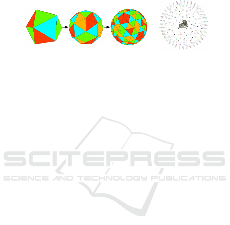
Figure 2: (a) Icosaheadron and its recursive subdivision to approximate a sphere for taking snapshots. The camera is positioned
at the center of each face and is pointed towards the 3D model kept at the center of the polyhedron. (b) The generated point
cloud from the triangulation on the resulted snapshots and the position of the virtual cameras.
unique sequence of three numbers, λ
1
, λ
2
, λ
3
≥ 0 such
that λ
1
+ λ
2
+ λ
3
= 1 and p = λ
1
v
1
+ λ
2
v
2
+ λ
3
v
3
.
(λ
1
, λ
2
, λ
3
) is called the Barycentric coordinates of
the point p with respect to the triangle (v
1
, v
2
, v
3
).
With these coefficients for linear interpolation, the
textured pixel of any point p lying inside the face
with vertices v
1
, v
2
, v
3
is given by I(p
0
), where p
0
=
λ
1
t
1
+ λ
2
t
2
+ λ
3
t
3
and λ
i
are the Barycentric coordi-
nates of p with respect to the vertices v
i
s.
Note the mapping p 7→ p
0
, from the 3D point p
to the 2D image location p
0
, inherently present in a
textured 3D model. We just leverage this information
for augmenting 2D feature descriptors to 3D points.
Also, since Barycentric coordinates are unique for
a point lying inside the triangle, (λ
1
, λ
2
, λ
3
) are
the barycentric coordinates of p
0
with respect to
(t
1
, t
2
, t
3
) as well, and the mapping between the 3D
point p and 2d point p
0
is one-to-one, related by
their barycentric coordinates in their respective faces.
We use this inverse map p
0
7→ p to assign features
extracted in the texture-image I to the 3D points,
thereby having a feature augmented model m. The
algorithm is described in Algorithm 1.
3.2 Snapshot based Training
In this approach instead of relying on the texture map
directly, we consider the real visual aspects of the
model. This is similar to the traditional offline train-
ing stage performed on real objects with a key differ-
ence. Because of the availability of 3D models with
us, we are free to choose virtual snapshot models of
our choice and experiment with the outcome with re-
spect to the quality of the model being generated.
Given a 3D model, we first take virtual snapshots
from several directions based on a snapshot model.
We then perform triangulation on the collection of
features in the snapshots to get 3D points. The set
of view dependent feature descriptors corresponding
to a 3D point is clustered using Mean Shift clustering
in the descriptor space and assigned to the 3D point,
thereby providing us a feature augmented 3D model.
Because of the richness of our snapshot model, we
only consider the points which are seen in atleast 5
different snapshots giving us a set of robust points in
terms of visibility.
Snapshot Model. In order to take maximum advan-
tage of the available 3D models, we intend to take
snapshots from every direction to cover all viewing
angles. This can be approximated by placing the
model in the origin and pointing the camera towards
the model from a set of uniformly discretized rotation
angles. One of the way of achieving this is to use
the faces (or vertices) a tesselated sphere built from
a regular polyhedrons as viewpoint locations. Since
the largest convex regular polyhedron is icosahead-
ron with 20 faces, we use a tesselated icosaheadron
to approximate the sphere. The tesselation parameter
controls how many times the triangles of the original
icosaheadron are divided to approximate the sphere.
Tesselation parameter of n would divide each triangle
into four equilateral triangles recursively for n times.
We generate feature augmented models with snap-
shots taken with tesselation level 0, 1 and 2 which
gives a total of 20, 80 and 320 snapshots respectively
as shown in Figure 2a. The trained models from all
such sets are considered for evaluation.
In a snapshot, the 3d model is rendered in a white
background with a directional headlight located at the
center of the camera, and with other default rendering
settings of Visualization Toolkit (VTK). One exam-
ple of the reconstructed point cloud together with the
position of the virtual cameras is shown in Figure 2b.
4 RECOGNITION FROM A
SINGLE IMAGE
This is the online stage which involves object recog-
nition in a calibrated query image I using a set of
Trained 3D models M = {m
r
}, m
r
= {V
r
}. The pres-
Feature-augmented Trained Models for 6DOF Object Recognition and Camera Calibration
635

ence of 2D feature de-scriptors in our 3D model
makes 6DOF recognition extremely easy. Here we
briefly describe the two popular techniques we used
for our evaluation for the shake of completeness.
PNP+RANSAC. This is the simplest and well stud-
ied form of object recognition. Features are extracted
in a query image and matched against that in our
trained models to get a set of 3D to 2D correspon-
dences. These 3D - 2D point correspondences are
used to compute the pose by one of the dedicated
Perspective-n-Point problem (PnP) methods [Demen-
thon and Davis, 1995, Lepetit et al., 2009]. The PnP
procedure is carried under the RANSAC scheme. Ob-
ject is said to be recognized, if PnP converges with an
error under a threshold in a fixed number of RANSAC
iterations.
MOPED. Our main online recognition stage is built
upon MOPED [Collet Romea et al., 2011], one of the
most robust framework for object recognition. Fol-
lowing 7 steps are performed in sequence: Feature
extraction, Feature matching, Feature clustering, Hy-
pothesis generation, Cluster clustering, Pose refine-
ment and Pose recombination. The notable addition
of MOPED framework is the clustering of the features
in the image space (for removing matching outliers)
and clustering of the object hypothesis in a common
coordinate space (for handling multiple instances).
Readers are referred to the original paper for more
details.
5 SIMULTANEOUS CAMERA
CALIBRATION
When the camera parameters of the query image is not
known we use the 3D - 2D correspondences to per-
form camera calibration instead of solving for PnP. As
a result, for uncalibrated images, our trained model
can be directly used as a standard marker for perform-
ing calibration. Because of the presence of large num-
ber of outliers, the calibration procedure needs to be
performed under RANSAC with a large number of it-
erations. This is not a concern here as we consider
a single known model instead of a big database. We
described the procedure used in the following para-
graphs.
Initialization. We assume a simple linear projec-
tion model in the first step for calibration. In this
model, a 3D point X
i
and its projection 2D point x
i
is related by,
λ
i
x
i
= PX
i
,
(1)
where P = K[R t], K is the intrinsic matrix and
[R t] is the extrinsic matrix with R as a 3 x 3 rotation
matrix and t as a 3 x 1 vector denoting the translation.
Our aim here is to find the parameters P and hence
K, R,t from a given set of X
i
↔ x
i
correspondences.
System of equations of the form 1 for unknown P
and λ
i
is well studied and can be solved by the algo-
rithm DLT. To find the matrix K and R, we do a RQ
decomposition of first 3 x 3 submatrix of P.
Maximum Likelihood Estimation. To incorporate
distortion along with the projection and to overall re-
fine our intrinsics obtained in the section above, we
find maximum likelihood estimate of the parameters
by minimizing the function:
∑
i
||x
i
− P
K,R,t,D
(X
i
)||
2
(2)
where K, R and t are the intrinsics, rotation and
translation respectively as defined above, and D =
{k1, k2, k3, k4} is the set of non-linear distortion co-
efficients. P (X
i
) is the projection of X
i
including the
non-linear distortion with the above parameters. This
is a nonlinear minimization problem, which is solved
with the Levenberg-Marquardt (LM) Algorithm. As
an initial guess of the LM algorithm, we take D = 0,
and K, R and t as obtained in the initialization step.
6 EVALUATIONS
6.1 Experimental Settings
Model Acquisition. We acquired 3D models using
a light weight 3D scanner of 3Digify [3Digify, 2015]
consisting of two household cameras and a projec-
tor. This scanner acquires the 3D geometry by pro-
jecting a fringe pattern and captures the distortion of
this pattern over the object surface with two cameras.
In the end we acquired high resolution textured 3D
models of 7 different real objects of different types;
namely Lion, Totem, Energy-drink, Matriochka,
Milk-carton, Whitener and Russian-cup. Out of
these, Milk-carton has dominant planar surfaces with
synthetic texture and resembles planar models and
surfaces with synthetic textures. Lion and Totem on
the other hand have very complex shape with nat-
ural texture. Energy-drink and Whitener resembles
synthetically textured cylindrical household models.
Matriochka and Russian-cup form their own category
with their partially oval shapes.
Methods. We used the SIFT-GPU [Wu, 2007] as
our main feature extraction algorithm. In our snapshot
based training, we used the default rendering param-
eters of Visualisation Tookit (VTK) for taking virtual
snapshots and subsequently, VisualSFM toolkit which
VISAPP 2016 - International Conference on Computer Vision Theory and Applications
636

Lion
Totem
Energy-
drink
Matriochka
Milk-
carton
Whitener
Russian-
cup
600 800 1000 1200 1400 1600 1800 2000 2200
Width resolution
0.3
0.4
0.5
0.6
0.7
0.8
0.9
1.0
Recognition recall
base
snap1
snap2
tmap
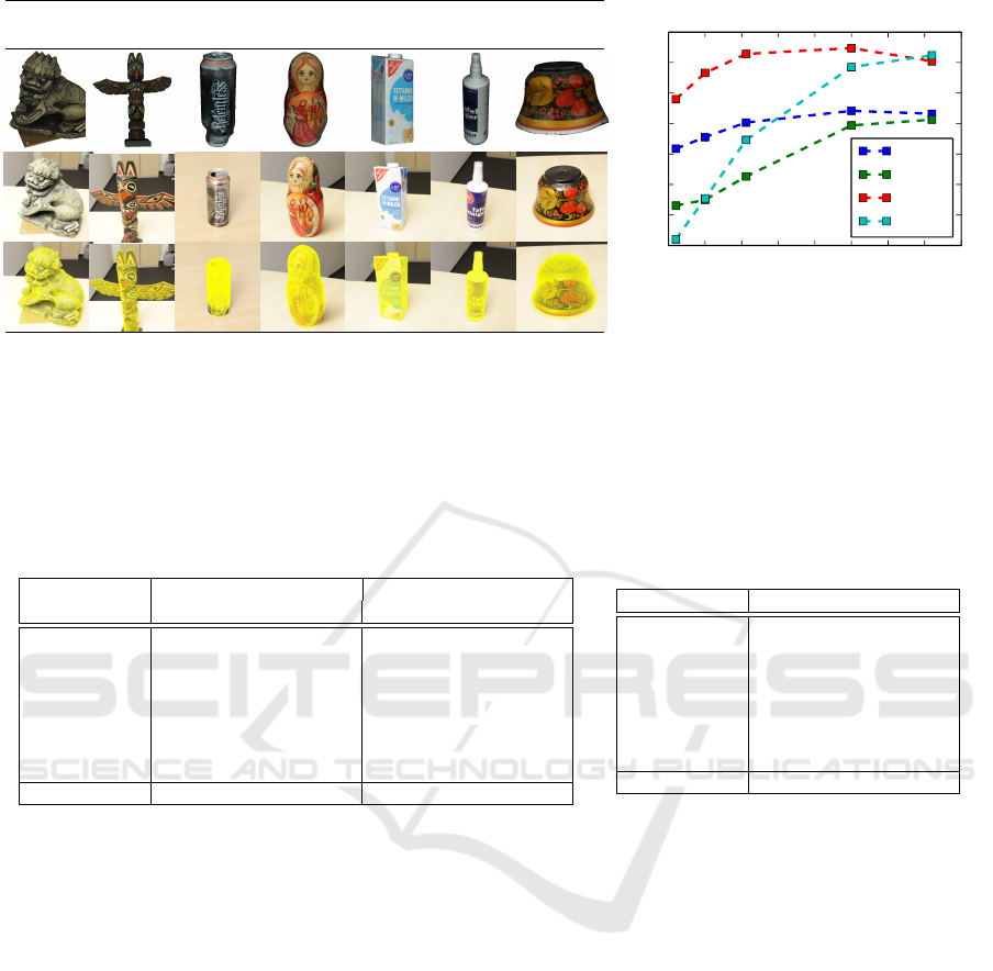
Figure 3: (Left) Models that are considered for evaluations. The first row shows the 7 acquired CAD models. The second
row shows the images of the real objects of the corresponding models. The third row shows result of 6DOF recognition where
mesh from the CAD models are reprojected on to the 2D images using the extrinsics found. Note that the images are zoomed
towards the model for better visualization. (Right) Comparison of recognition recall of our methods with the existing base
whose trained model is obtained by the manual way of taking pictures, segmenting and performing SFM.
Table 1: (Left) Comparison of object recognition recall with MOPED of our trained model. ‘All Resolution’ includes the
results from the width-resolution 640, 800, 1024, 1600 and 2040 pixels. We achieved best results in our two highest resolutions
(of width 1600 and 2040) which are shown separately under ‘Largest Resolutions’. (Right) Object recognition recall using
PNP+RANSAC with images of width-resolution 1600 and 2040.
All Resolutions Largest Resolutions
Models snap1 snap2 tmap snap1 snap2 tmap
Milk-carton 0.79 0.88 0.71 0.93 1.00 0.95
Totem 0.44 0.83 0.21 0.40 0.73 0.31
Lion 0.56 0.89 0.63 0.72 0.93 0.90
Whitener 0.34 0.48 0.63 0.57 0.82 0.80
Russian-cup 0.45 0.42 0.45 0.95 0.91 1.00
Energy-drink 0.57 0.52 0.54 0.93 0.79 0.88
Matriochka 0.63 0.58 0.62 1.00 1.00 1.00
Average 0.55 0.79 0.57 0.73 0.89 0.84
Models snap1 snap2 tmap
Milk-carton 0.93 0.83 0.55
Totem 0.32 0.82 0.24
Lion 0.71 0.83 0.72
Whitener 0.15 0.15 0.15
Russian-cup 0.41 0.32 0.36
Energy-drink 0.67 0.76 0.59
Matriochka 0.82 0.84 0.61
Average 0.64 0.77 0.59
uses Multicore Bundle Adjustment [Wu et al., 2011],
as our triangulation tool.
For each of the 7 3D models, we obtained the
feature augmented models from texture-map based
method (Section 3.1) which we call tmap, and snap-
shots based method (Section 3.2) with virtual snap-
shots taken with a tesselation level of 1 and 2, and
call them snap1, snap2 respectively.
Query Image Dataset. We captured more than 100
images for each of the 7 objects keeping them at var-
ious distance from the camera varying from 30 cms
to 100 cms. Out of them we generated images of dif-
ferent resolutions width of 640, 800, 1024, 1600 and
2040 pixels (keeping the aspect ratio same). There-
fore, each object in our object database is associated
with more than 500 images with the total of more than
3500 images for the entire dataset.
6.2 Evaluation of Trained Models for
Recognition
In this set of experiments we evaluate our trained
models in terms of their ability to be recognized by
an online recognition stage as discussed in Section
4. Because of its robustness, we chose the recogni-
tion method based on MOPED to compare the results
of the different variation of our algorithm, namely
snap1, snap2 and tmap.
We use the Quality Score (Q-Score) defined in
[Collet Romea et al., 2011] to consider an object to
be recognized in its corresponding image. Q-Score
is a correspondence-number independent score of a
recognition hypothesis based on Cauchy distribution
with a lower bound 0 and upper bound as the number
of correspondences. In our case an object is consid-
ered to be recognized in its associated captured image
when MOPED converges to a Q-Score of 5.
The comparison of our different methods can be
Feature-augmented Trained Models for 6DOF Object Recognition and Camera Calibration
637

0.0 0.2 0.4 0.6 0.8 1.0 1.2
RMS reprojection eror
0.0
0.5
1.0
1.5
2.0
2.5
3.0
Normalized frequency
txtmap
snap2
snap1
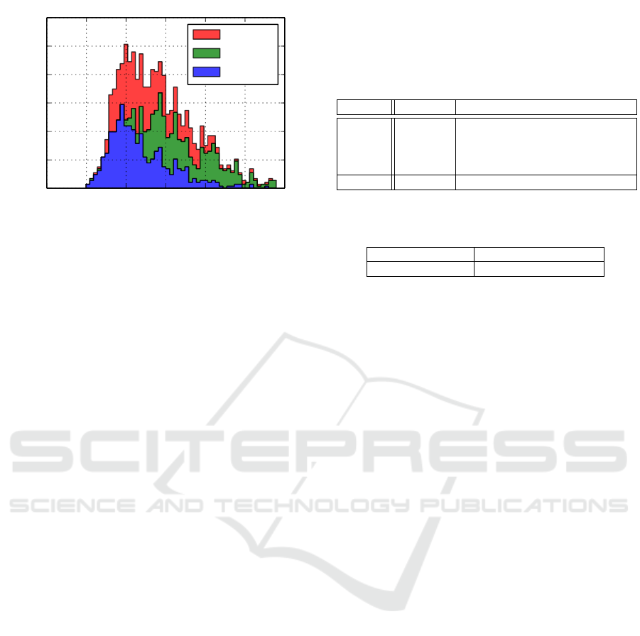
Figure 4: RMS reprojection error (pixels) from our calibra-
tion technique using the trained model. The histograms are
stacked over each other for better visualization. Best viewed
in color.
found in Table 1 (Left). As expected the highest
recognition recall is found with snap2 which consid-
ers 320 virtual snapshots. The second overall recogni-
tion recall is achieved by our very simple texture-map
based method tmap and outperforms snap1 which
considers 80 virtual snapshots.
Comparison with the Baseline. In this experiment
we compare our methods with the traditional man-
ual way of creating feature augmented models from
real objects. For this purpose we use our most com-
plexly shaped object - Lion for evaluation. The base-
line feature-augmented model (base) of Lion is cre-
ated by manually taking 50 high quality images from
different directions. Each of the images is then seg-
mented for the object by manually creating a mask
around the object in the image to remove background
scene. These segmented images are then used for re-
construction to obtain sparse 3D point cloud with 3D
points augmented with the clustered view dependent
feature descriptors. The result of the final evaluation
is shown in Figure 3 (Right). Our snap2 comes out
superior in all resolutions here as well. In higher res-
olution images our method tmap performs better than
the base. This is because the scale of the query im-
ages matches to the scale of the texture map at the
larger resolution.
Online Algorithm Independence. To show that
our trained model is independent of the online stage,
we perform and compare the results from a simple
PNP+RANSAC (Section 4) based online recognition
stage and compared with that of MOPED. Here we
chose a RANSAC scheme with 500 iteration, 80%
confidence and reprojection error threshold as 2 pix-
els. Objects are said to be recognized when the
RANSAC converges with the above settings. The
Table 2: Comparison of calibration result of [Bouguet,
2008] and our method using the augmented model of
Lion+snap2 and images of size 2040x1360. ‘sample’ is
the calibration results of one particular image; ‘mean’ and
‘deviation’ are the respective statistical functions on the cal-
ibration results over all the images.
params Bouguet sample mean deviation
fx 1364.00 1360.76 1368.83 68.54
fy 1368.31 1364.41 1368.49 67.50
cx 999.34 1005.48 1039.27 78.64
cy 690.20 715.21 663.81 50.99
rms 0.62 0.51 0.58 0.10
Table 3: Average RMS reprojection error of our different
models.
sna1 snap2 tmap
avg RMS (pixels) 0.47 0.69 0.53
results of the recognition recall with the images of
width-resolution 1600 and 2040 are shown in Table
1 (Right). Because of no outlier detection a-priori of
RANSAC we get comparably low recognition recall
compared to MOPED. But an average of recognition
recall of more than 50% on a simple PNP+RANSAC
based recognition verifies that our trained model is in-
dependent of the online recognition algorithm.
6.3 Evaluation of Trained Models for
Calibration
In this set of experiments we evaluate our trained
models in terms of their ability to be used as a cal-
ibration rig. We used the object Lion for this pur-
pose because of its highly complex shape which em-
phasizes the fact that our technique is different than
most of the popular available calibration technique
which depends on the planer nature of the calibration
rig [Bouguet, 2008,Heikkila and Silven, 1997,Zhang,
1999]. As the model is fixed and known, we chose a
large RANSAC iteration of 1000 and an RMS error
threshold of 2 pixels in all our experiments for cali-
bration.
Variation and Stability. Around 50 images of Lion
were taken from random direction with a fixed fo-
cus camera. Without changing the focus and other
settings of the same camera, 15 images of stan-
dard chessboard were taken as well. The images
of the chessboard were then used for calibration us-
ing the popular Bouguet’s Camera Calibration Tool-
box [Bouguet, 2008] for comparison. Because of its
higher detection rate in PNP+RANSAC scheme we
considered the the trained model snap2 for perform-
ing calibration on the images of Lion for an exten-
sive evaluation of variation of the intrinsics (Equation
VISAPP 2016 - International Conference on Computer Vision Theory and Applications
638

1). Each image of Lion was calibrated separately us-
ing our simple DLT+MLE method (Section 5) under
RANSAC. The mean and the standard deviation of the
calibration results of all the images are compared and
provided in Table 2. It is observed that, the RMS re-
projection error of our technique is smaller than that
of [Bouguet, 2008] in most of the cases. Because
we only take one image for calibration, our result is
tightly coupled with that particular image which is re-
flected with the low RMS error and moderate standard
deviation over all the images.
RMS Error Analysis. In the next experiment we
make an analysis over the RMS reprojection error
over images of various types, sizes and focal lengths
for all our modelling methods. For each model snap1,
snap2 and tmap, we calibrated all the images of Lion
from ‘query image dataset’ (more than 500 images
with width-resolution 640, 800, 1024, 1600 and 2040
pixels) and collected their RMS error. The distribu-
tion of RMS error is represented as histogram in Fig-
ure 4 and the mean RMS error is provided in Table
3. As shown, though the error from our method is
spreaded over a good spectrum because of the various
types of images used, our mean RMS error is small
which makes our method a quick and reliable tool for
camera calibration where an extreme accuracy is not
a concern.
7 CONCLUSION
We have presented methods for creating feature-
augmented models from CAD models for the purpose
of 6DOF object recognition and camera calibration.
The fully automatic procedure produces models that
are capable of being recognized in single image with
high accuracy with different flavours of online stage,
and as a natural marker for the purpose of camera cal-
ibration.
In the future we look forward to consider view de-
pendent global features (Eg. 2D shape context) to be
computed on our virtual snapshots in an attempt to
match them in query images. In this way we plan to
include geometric information along with the texture
in our trained models.
ACKNOWLEDGEMENTS
This work was partially funded by the BMBF project
DYNAMICS (01IW15003).
REFERENCES
3Digify (2015). 3digify, http://3digify.com/.
Aldoma, A., Tombari, F., Rusu, R., and Vincze, M. (2012).
Our-cvfh oriented, unique and repeatable clustered
viewpoint feature histogram for object recognition
and 6dof pose estimation. In Pinz, A., Pock, T.,
Bischof, H., and Leberl, F., editors, Pattern Recogni-
tion, volume 7476 of Lecture Notes in Computer Sci-
ence, pages 113–122. Springer Berlin Heidelberg.
Bouguet, J. Y. (2008). Camera cal-
ibration toolbox for Matlab,
http://www.vision.caltech.edu/bouguetj/calib doc/.
Collet Romea, A., Martinez Torres, M., and Srinivasa, S.
(2011). The moped framework: Object recognition
and pose estimation for manipulation. International
Journal of Robotics Research, 30(10):1284 – 1306.
Collet Romea, A. and Srinivasa, S. (2010). Efficient multi-
view object recognition and full pose estimation. In
2010 IEEE International Conference on Robotics and
Automation (ICRA 2010).
D’Apuzzo, N. (2006). Overview of 3d surface digitization
technologies in europe. In Electronic Imaging 2006,
pages 605605–605605. International Society for Op-
tics and Photonics.
Dementhon, D. and Davis, L. (1995). Model-based ob-
ject pose in 25 lines of code. International Journal
of Computer Vision, 15(1-2):123–141.
Hao, Q., Cai, R., Li, Z., Zhang, L., Pang, Y., Wu, F., and
Rui, Y. (2013). Efficient 2d-to-3d correspondence fil-
tering for scalable 3d object recognition. In Computer
Vision and Pattern Recognition (CVPR), 2013 IEEE
Conference on, pages 899–906.
Heikkila, J. and Silven, O. (1997). A four-step camera cal-
ibration procedure with implicit image correction. In
Computer Vision and Pattern Recognition, 1997. Pro-
ceedings., 1997 IEEE Computer Society Conference
on, pages 1106–1112.
Irschara, A., Zach, C., Frahm, J.-M., and Bischof, H.
(2009). From structure-from-motion point clouds to
fast location recognition. In Computer Vision and
Pattern Recognition, 2009. CVPR 2009. IEEE Con-
ference on, pages 2599–2606.
Lepetit, V., Moreno-Noguer, F., and Fua, P. (2009). Epnp:
An accurate o(n) solution to the pnp problem. Int. J.
Comput. Vision, 81(2):155–166.
Lowe, D. (2004). Distinctive image features from scale-
invariant keypoints. International Journal of Com-
puter Vision, 60(2):91–110.
Rusu, R., Bradski, G., Thibaux, R., and Hsu, J. (2010). Fast
3d recognition and pose using the viewpoint feature
histogram. In Intelligent Robots and Systems (IROS),
2010 IEEE/RSJ International Conference on, pages
2155–2162.
Skrypnyk, I. and Lowe, D. (2004). Scene modelling, recog-
nition and tracking with invariant image features. In
Mixed and Augmented Reality, 2004. ISMAR 2004.
Third IEEE and ACM International Symposium on,
pages 110–119.
Feature-augmented Trained Models for 6DOF Object Recognition and Camera Calibration
639

Tombari, F., Salti, S., and Di Stefano, L. (2010). Unique
signatures of histograms for local surface descrip-
tion. In Computer Vision–ECCV 2010, pages 356–
369. Springer.
Wu, C. (2007). SiftGPU: A GPU implementa-
tion of scale invariant feature transform (SIFT).
http://cs.unc.edu/ ccwu/siftgpu.
Wu, C., Agarwal, S., Curless, B., and Seitz, S. (2011). Mul-
ticore bundle adjustment. In Computer Vision and Pat-
tern Recognition (CVPR), 2011 IEEE Conference on,
pages 3057–3064.
Zhang, Z. (1999). Flexible camera calibration by viewing
a plane from unknown orientations. In Computer Vi-
sion, 1999. The Proceedings of the Seventh IEEE In-
ternational Conference on, volume 1, pages 666–673.
IEEE.
VISAPP 2016 - International Conference on Computer Vision Theory and Applications
640