Skin Surface Reconstruction and 3D Vessels Segmentation in Speckle
Variance Optical Coherence Tomography
Marco Manfredi
1
, Costantino Grana
1
and Giovanni Pellacani
2
1
Department of Engineering“Enzo Ferrari”, University of Modena and Reggio Emilia, Modena, Italy
2
Department of Dermatology, University of Modena and Reggio Emilia, Modena, Italy
Keywords:
Medical Imaging, 3D Reconstruction, Vessel Segmentation, Visualization.
Abstract:
In this paper we present a method for in vivo surface reconstruction and 3D vessels segmentation from Speckle-
Variance Optical Coherence Tomography imaging, applied to dermatology. This novel technology allows
us to capture motion underneath the skin surface revealing the presence of blood vessels. Standard OCT
visualization techniques are inappropriate for this new source of information, that is crucial in early skin
cancer diagnosis. We investigate 3D reconstruction techniques for better visualization of both the external and
internal structure of skin lesions, as a tool to help clinicians in the task of qualitative tumor evaluation.
1 INTRODUCTION
Optical Coherence Tomography (OCT) is a laser-
based imaging modality that is capable of provid-
ing detailed pictures of sub-surface tissue microstruc-
ture to a depth of 1 mm+ in real time, and has been
very successfully applied to imaging the eye (Huang
et al., 1991; Leitgeb et al., 2003). OCT was first ap-
plied to imaging skin as early as 1997 (Welzel et al.,
1997). However, image quality and scanning speed
remained insufficient until multi-beam OCT was de-
veloped (Holmes et al., 2008). Multi-beam OCT com-
bines OCT data from multiple laser beams focused at
slightly different depths in the tissue, scanned simul-
taneously through the region of interest.
“Standard” OCT relies on the small variations in
intensity of back-scattered light from different tissue
cellular microstructures to reveal the tissue morphol-
ogy (Huang et al., 1991). The resulting contrast be-
tween some tissue types can be quite low, and so there
has been continued interest in development of tech-
niques with the potential of extracting further clini-
cally useful information from the OCT data (Schmitz
et al., 2013; Hitzenberger and Fercher, 1999).
One technique of great promise is speckle-
variance OCT (SV-OCT) (Mariampillai et al., 2008;
Mahmud et al., 2013; De Carvalho et al., 2015).
Briefly, SV-OCT involves rapidly repeating OCT
scans, and analyzing the statistics of the OCT sig-
nal, to detect regions of the OCT images which have
changed between these successive scans. Most of the
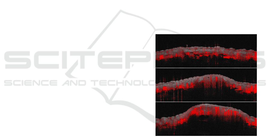
Figure 1: Sample slices from a Dynamic OCT scan. The
redness information highlights motion underneath the skin
surface, and it is used to detect blood vessels.
scanned tissue is unchanged, but any blood flowing
produces small changes in the SV-OCT data that are
detectable, thereby revealing the presence of blood
vessels and capillaries. SV-OCT allows the visu-
alization of vessels as small as ~20µm in diameter
without the use of contrast agents. The analysis of
vascular networks is fundamental because tumors re-
quire access to blood vessels for oxygen and nutrients,
producing abnormalities in vessel morphology (Jain,
2001).
In our images, the areas of motion are highlighted
in red, with the most intense red corresponding to the
234
Manfredi, M., Grana, C. and Pellacani, G.
Skin Surface Reconstruction and 3D Vessels Segmentation in Speckle Variance Optical Coherence Tomography.
DOI: 10.5220/0005758702340240
In Proceedings of the 11th Joint Conference on Computer Vision, Imaging and Computer Graphics Theory and Applications (VISIGRAPP 2016) - Volume 4: VISAPP, pages 234-240
ISBN: 978-989-758-175-5
Copyright
c
2016 by SCITEPRESS – Science and Technology Publications, Lda. All rights reserved
strongest motion. See Figure 1 for examples. We use
the term “dynamic OCT” to distinguish the detected
motion from the standard OCT image data, which we
refer to as “structural OCT”.
Structural OCT visualization software is inca-
pable of showing the vascular structures in an effec-
tive way, since they are built to work on structural
OCT data. The potential informativeness of blood
vessel detection has to be investigated using new vi-
sualization methods.
This paper focuses on the visualization of dy-
namic OCT images by means of 3D reconstruction
algorithms to capture external and internal structures
of skin lesions. The novelty of the work consists
in proposing an image analysis pipeline to deal with
novel dynamic OCT data, with the goal of presenting
it at best for qualitative in vivo tumor diagnosis.
2 RELATED WORK
In the following we will present notable works on the
topics of OCT image analysis and vessel segmenta-
tion both in 2D and 3D.
A lot of work in recent years has been done in reti-
nal vessel segmentation (Soares et al., 2006; Niemei-
jer et al., 2008). In (Soares et al., 2006) multi-scale
Morlet Wavelet transform responses are used as fea-
tures in a binary classification approach to highlight
the presence of vessels of different diameters. 3D
OCT volumes are used in (Niemeijer et al., 2008)
to obtain a 2D projection image from a segmented
layer for which the contrast between the vascular sil-
houettes and background is highest. The high con-
trast between foreground and background allows their
method to effectively segment the vessel silhouettes
using a supervised pixel-based approach. Differently
from retinal OCT images, the vascular network of
skin lesions has a 3D structure that can not be cap-
tured by a single 2D view. We have to tackle 3D
vascular segmentation. 3D vascular segmentation and
reconstruction have been applied for years to brain
imaging (Wu et al., 2011; Manniesing et al., 2006;
Lesage et al., 2009; Tankyevych et al., 2009). In (Wu
et al., 2011) images are cleaned with an anisotropic
filtering, followed by skin and bones removal. Level
sets are then applied for the segmentation of the
vascular network. Their work then focuses on re-
construction of the segmented vessels demonstrating
the effectiveness of an ellipse model assumption and
proposing a solution to the branching problem. A no-
table difference between Computed Tomography An-
giography or Magnetic Resonance Angiography im-
ages used in these works and OCT imaging, is that
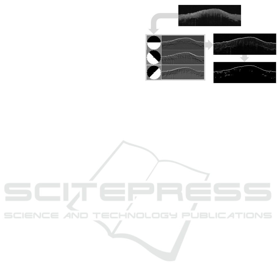
Input image
Convolution
Maximum Response
After non-maxima suppression
Figure 2: The filtering procedure. Circular kernels are ap-
plied to highlight the surface boundary followed by a non-
maxima suppression step to obtain a single response per
edge.
OCT has a limited penetration depth (about 1mm).
As can be seen in Figure 1, only superficial structures
are detected, leading to potentially incomplete vascu-
lar networks. Furthermore, the amount of noise in
dynamic OCT images increases when moving deeper
in the tissue. A straight-forward application of the
methods listed above is not possible for dynamic OCT
imaging and alternative solutions must be explored.
A preliminary work on SV-OCT, proposed
in (Conroy et al., 2012), tackles the problem of quan-
titative measurements of vascular structures. They
propose to measure quantitative metrics to charac-
terize the vessel morphology, and they validate their
approach on mice (comparing healthy and tumor-
bearing mice). Our work differs from theirs as: (i)
the subjects of our analysis are humans and not mice,
(ii) they minimize bulk motions with a customized
holder, while our images are captured with a hand-
held device (resulting in higher levels of noise) and
(iii) we detail the image analysis pipeline to achieve
clear visualization of the vascular networks and for
the reconstruction of the lesion surface.
3 SURFACE RECONSTRUCTION
This section details the algorithm for the reconstruc-
tion of the top surface of the skin. Having the 3D
shape of the surface allows a better visualization of
the vascular networks that can be analyzed at uniform
depths from the outer surface, as shown in Section 4.
Horizontal slices of the epidermis can thus follow the
shape of the interested region helping the clinicians in
the diagnosis. The input data are 121 RGB images of
size 1370×460 coming from the OCT scanner, rep-
resenting vertical slices of skin, covering an area of
approximate size of 5mm×5mm. The expected out-
Skin Surface Reconstruction and 3D Vessels Segmentation in Speckle Variance Optical Coherence Tomography
235

0
50
100
150
200
250
300
350
400
450
500
0 200 400 600 800 1000 1200
Height of the surface
Spline
Data points
Subsampling
Figure 3: Reconstructing a smooth surface one slice at a time: the original data points (red) are subsampled (black) and after
a median filter they are used as reference points for a second-order spline curve fitting (cyan).
put is an image of size 1370×121 where each element
contains the height of the reconstructed surface. Since
the scanned area of skin is squared, a final resizing
step to 1370×1370 is applied to compensate the un-
even horizontal/vertical resolution of the scanner.
The challenges of this task are represented by the
size of the input data (about 220MB per scan) and by
the noise of the input images. Since the scanner is
hand-held by the clinician, misalignments are often
present between adjacent slices. Some slices from a
scan are presented in Figure 1.
To reconstruct the surface, gray level images are
used since color information (i.e. redness) only define
the vascular structure underneath the epidermis.
Our approach starts by analyzing each slice sepa-
rately, finding a rough estimation of the height of the
surface. Inspired by (Arbelaez et al., 2011), that suc-
cessfully proposed a method for contour detection in
natural images, given a slice a collection of N circular
filters at different orientations is applied to highlight
the boundary of the skin.
A fixed size of 25×25 is chosen for all kernels,
which has been proven to be robust to the noise level
of the input data. The N convolutions are reduced to
one image where each pixel is the maximum response
over all filters. The higher the number of filters N,
the more accurate the result is because the orientation
quantization is lower. However, we found that in prac-
tice using 3 filters produces an accurate response for
the surface. The orientations of the 3 filters are -45°,
0° and 45°. The filtering step produces a smooth re-
sponse over the skin boundary, where we would like
to have a thin line following the surface; non-maxima
suppression is thus applied (Canny, 1986). The filter-
ing pipeline is summarized in Figure 2.
To obtain a unique response for each column of
the slice, we select the topmost pixel the has a re-
sponse greater than a threshold T . The choice of T has
been done experimentally (T = 0.1 where the maxi-
mum response is 1.0) but as it can be seen in the last
picture of Figure 2, the very high contrast between the
boundary and the rest of the image makes the choice
of T quite robust to noise.
A tradeoff between reconstruction accuracy and
smoothness is unavoidable. A very accurate recon-
struction would maintain every small curvature of the
skin, at the cost of losing some robustness to noise
where hair or other artifacts are present. Smoothing
the surface too much could create discrepancies be-
tween the actual surface and the reconstruction, that
we would like to avoid. Since the clinicians do not
need a fine detail reconstruction, we decided to do a
subsampling of the available data points (found after
the threshold). Taking less points does not prevent
noisy data to be selected and for this reason we apply
a median filter along the line. This step allows to re-
move noisy peaks and drops. Finally, a second-order
spline curve fitting is applied to smoothly connect the
available reference points. The subsampling step has
been set to 15, the length of the median filter to 5. In
Figure 3 the same slice of Figure 2 is analyzed using
the described algorithm.
At this point we have independently reconstructed
121 curves (one per slice), what we need to do is
to enforce smoothness along the perpendicular direc-
tion to the slices. The same pipeline of algorithms
is applied vertically: (i) subsampling (step=3 in this
case) (ii) median filter with size 5 to remove drops
and peaks and (iii) spline interpolation. The only dif-
ference here is that the surface must be stretched to
squared proportions for the final result. In Figure 4 the
contributions of the slice-wise and vertical smoothing
are highlighted. Most of the unwanted artifacts are re-
moved by the first step, but the vertical smoothing is
still required to remove bigger discontinuities and to
smoothly connect adjacent slices.
The filtering and the spline fitting steps, that are
the most computationally expensive, have been par-
allelized (since each slice is analyzed independently).
The running time of the complete pipeline on a mod-
ern pc (Intel-i7 4790k) is of 3-4 seconds.
Once the shape of the surface has been recon-
structed, textures are applied on it using the input
data. We can thus obtain a 3D visualization of the
surface, presented in Figure 5.
VISAPP 2016 - International Conference on Computer Vision Theory and Applications
236
1
2
3
a)
b)
c)
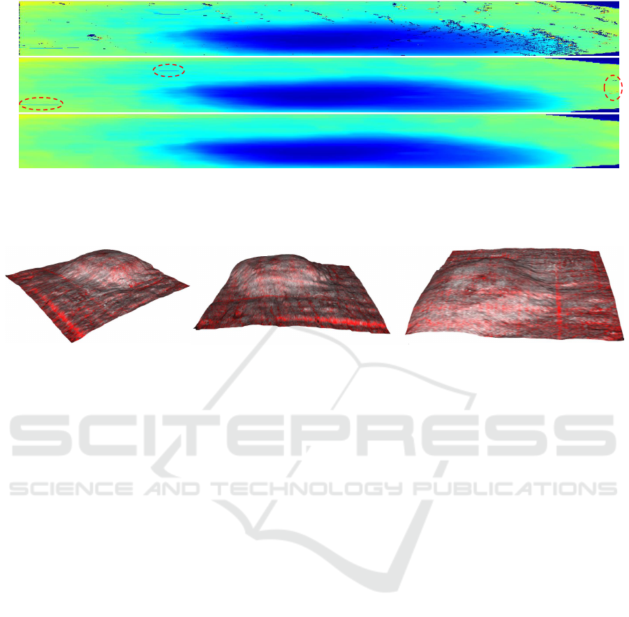
Figure 4: Top view of the reconstructed surface, viewed in the original dimensions of 1370×121 (best viewed in color). The
color of the surface encodes the depth (blue=shallow, red=deep). In a) the surface after the filtering step is presented; drops
and peaks are evident. b) is the result after the horizontal subsampling and spline fitting. Some artifacts are still visible (e.g.
areas 1, 2 and 3) and are further corrected with the vertical smoothing step shown in c).
Figure 5: 3D visualization of the reconstructed surface from multiple views.
4 VESSELS VISUALIZATION
The novelty of the dynamic OCT over standard OCT
technologies resides in capturing motions underneath
the surface of the skin. This motion carries informa-
tion about blood flows, giving insights about the vas-
cular network. The visualization of the vascular net-
work is not trivial and we identified 3 ways of pre-
senting it to the clinician:
1. Horizontal view: vertical slices can be used to cre-
ate a top-view by sampling horizontal images that
better present the vascular network compared to
the partial information of each vertical slice sepa-
rately.
2. Depth preserving horizontal view: the horizontal
view can be enhanced by using the reconstructed
3D surface to sample data at uniform depths. We
thus obtain a horizontal view in which every point
is captured at the same depth from the surface.
The advantage of this solution compared to the
previous one becomes clear when analyzing par-
ticularly convex skin lesions.
3. 3D view: the most informative way of visualizing
the vascular network consist of 3D visualization.
Several problems have to be tackled to obtain a
realistic and clear view of the vessels, like the
removal of all non-vessel data. In the following
section we will detail the proposed procedure.
In Figure 6 a comparison of the three approaches
discussed above clearly highlights the improvements
in informativeness of the depth preserving horizontal
view and 3D view over the standard approach. The
convexity of the analyzed lesion leads the horizontal
view to fail in capturing the global vessel structure.
Although the depth preserving horizontal view solves
this problem, it still shows one layer at a time, while
the 3D view presents the complete vessel network.
4.1 3D Vessel Segmentation
Blood flow information is encoded as redness in the
dynamic OCT images, since only the detected motion
is colored while the rest of the image is gray-scale.
As can be seen in Figure 1, the red channel tends to
saturate in the presence of strong motion, while lower
values of the red channel are often caused by noise.
Since the OCT scanner is hand-held, any small shift
of the device or of the captured skin lesion is cap-
tured as a motion and reproduced as redness in the
corresponding areas. In the middle image of Figure 1,
red peaks caused by unintended motions are visible
on the left. As a consequence we have to design our
vessel reconstruction algorithm to cope with noisy de-
tections.
To remove all the data except the vessel network
we apply a threshold on the difference between the
red channel and the blue channel for each pixel in-
Skin Surface Reconstruction and 3D Vessels Segmentation in Speckle Variance Optical Coherence Tomography
237
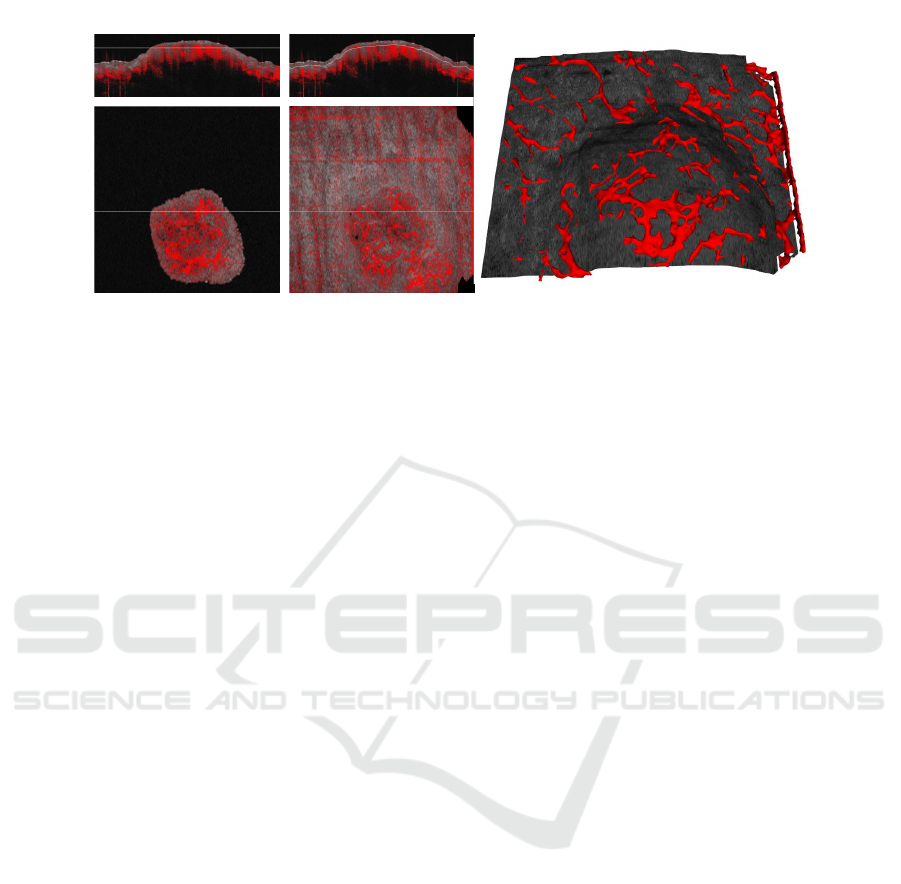
Horizontal view
Depth preserving
horizontal view
3D view
Figure 6: A comparison of three different solutions to present the vascular network. The surface extraction method, presented
in Section 3, allows to extract horizontal layers at constant depth from the surface, as shown in the middle images. On the
right, the 3D view detailed in Section 4.1 is reported.
dependently. The threshold is set empirically to 180
using tens of scans as reference.
On a regular scan, the point cloud that we ob-
tain is composed of tens of millions of points (the
scan of Figure 6 produces approximately 25 million
of points). To speed-up the reconstruction we sub-
sample the points using a step of 2 in each direction,
thus lowering the number of points to 3 millions. The
top-left picture of Figure 7 shows the resulting point
cloud from a top-view. Although the vascular struc-
ture is partially visible, the amount of noise is very
high.
3D Point Cloud Filtering
We design the filtering step as follows:
1. A 3D filter is computed using a cubic kernel cen-
tered at each point location, with side s1. The ra-
tio P
r
of red points inside the cube divided by its
volume is computed and only the red points with
P
r
≥ 50% are kept. This step removes isolated
points, while maintaining dense structures typical
of blood vessels.
2. Since the visualization of a blood vessel only re-
quires the rendering of the outer surface, all the
data points that lies in the inner part of a ves-
sel “tube” are in fact useless. Moreover, they
deeply impact the computational performance of
the mesh reconstruction algorithm. We thus re-
move all the data points whose neighbors (26
in total) entirely belong to the point cloud. For
this purpose, another cubic filter with side s2 = 1
(s2 < s1) is used.
Applying the previously described filters requires
the computation of the number of red points in cu-
bic boxes centered in each location of the point cloud
(we will refer to this number ad the mass of a box).
The size of the point cloud is easily computed from
the size of the scan images as 1370 × 460 × 1370 =
863374000 points. A trivial solution that iterates
through each point is unfeasible and leads to several
minutes of computation.
In the “integral images” approach, introduced in
(Viola and Jones, 2004), the integral image contains
at every point (x
0
, y
0
) the sum of all pixels with x < x
0
and y < y
0
. This allows to compute the sum of all val-
ues of a rectangle by combining just four values of the
integral image. In this paper we use an extension to
3D volumes (Grana et al., 2012) to compute in con-
stant time the mass of a box. To this aim the first step
is to extract the 3D integral point cloud.
Having p(c), the value of the point cloud at c
(p(c) = 1 or p(c) = 0), the 3D integral point cloud
ip(c) is defined as
ip(c) =
∑
x:x
k
<c
k
k=0,1,2
p(x) (1)
As for integral images, it is possible to compute the
3D integral point cloud by a single sweep over the
original data points, taking advance of the recursive
nature of the definition. In particular:
ip(c) = p(c) + ip(c
0
− 1, c
1
, c
2
) + ip(c
0
, c
1
− 1, c
2
)
− ip(c
0
− 1, c
1
− 1, c
2
) + ip(c
0
, c
1
, c
2
− 1)
− ip(c
0
− 1, c
1
, c
2
− 1) − ip(c
0
, c
1
− 1, c
2
− 1)
+ ip(c
0
− 1, c
1
− 1, c
2
− 1)
(2)
This assumes that the value of the 3D integral point
cloud is 0 whenever any of the coordinates is negative.
Given a 3D integral point cloud, the computation of
the mass within a box b = (l, h) is quite similar to the
VISAPP 2016 - International Conference on Computer Vision Theory and Applications
238

After subsampling
3.18 Millions Points
After filtering
1.04 Millions Points
After Delaunay Triangulation
After Laplacian Smoothing
Figure 7: From a point-cloud to a smooth 3D mesh: the
original (subsampled) point-cloud (top-left), the result after
filtering (top-right), the mesh generated using Delaunay tri-
angulation (bottom-left) and the final result (bottom-right).
All images are captured from a top-view camera, while in
the proposed visualization tool full 3D object manipulation
can be performed.
use of integral images for rectangle area calculations:
m(b) = ip(h
0
, h
1
, h
2
) − ip(l
0
− 1, h
1
, h
2
)
− ip(h
0
, l
1
− 1, h
2
) + ip(l
0
− 1, l
1
− 1, h
2
)
− ip(h
0
, h
1
, l
2
− 1) + ip(l
0
− 1, h
1
, l
2
− 1)
+ ip(h
0
, l
1
− 1, l
2
− 1) − ip(l
0
− 1, l
1
− 1, l
2
− 1)
(3)
This formulation holds, again assuming that ip(c) = 0
if c
k
= −1 for any k. The output of the filtering step
is shown in the top-right picture of Figure 7.
Mesh Reconstruction
The output of the filtering step is a cleaned 3D point
cloud with hollowed tubes representing blood vessels.
A standard solution when dealing with mesh recon-
struction from point cloud is the use of surface recon-
struction algorithms based on point normals, like the
algorithm proposed in (Kazhdan et al., 2006). How-
ever, the proximity between adjacent vessels and the
presence of holes/peaks complicates the computation
of reliable point normals.
For this reason we choose the Delaunay triangu-
lation, a technique that does not require any a pri-
ori knowledge of surface orientation normals. The
only parameter of the Delaunay triangulation, α, is
the maximum radius length used when triangulating
neighboring points. A too high value of α could
merge adjacent vessels (if the mutual distance be-
tween the two is comparable to α), a too low value
of α could create artifacts in the reconstruction and,
more specifically, holes. We set α so to obtain the
best trade-off between regularity of the vessels struc-
tures and the fine details representation. The result of
Delaunay triangulation is presented in the bottom-left
picture of Figure 7.
The visualization of the vascular network thus
obtained can be further improved with a Laplacian
smoothing step (Field, 1988), giving to the clinician a
more realistic view of the vessels appearance. The
final view presented to the user is presented in the
bottom-right picture of Figure 7.
5 CONCLUSION
In this paper we tackled the problem of visualization
of 3D surfaces and vascular networks from dynamic
OCT in vivo scans. This recently introduced tech-
nique for OCT imaging poses new challenges to the
image analysis community, that cannot be addressed
with straightforward application of previously pro-
posed methods. Our aim was to provide to the clini-
cian a tool for qualitative skin lesions evaluation. We
detailed a complete pipeline to deal with image noise,
surface reconstruction, vessel segmentation and 3D
visualization.
ACKNOWLEDGEMENT
The research leading to these results has received
funding from the European Union’s Competitiveness
and Innovation framework Programme CIP 2007-
2013. Project Name: ADVANCE, reference: 621015.
REFERENCES
Arbelaez, P., Maire, M., Fowlkes, C., and Malik, J. (2011).
Contour detection and hierarchical image segmen-
tation. IEEE Trans. Pattern Anal. Mach. Intell.,
33(5):898–916.
Canny, J. (1986). A computational approach to edge detec-
tion. Pattern Analysis and Machine Intelligence, IEEE
Transactions on, (6):679–698.
Conroy, L., DaCosta, R. S., and Vitkin, I. A. (2012). Quan-
tifying tissue microvasculature with speckle vari-
ance optical coherence tomography. Optics letters,
37(15):3180–3182.
Skin Surface Reconstruction and 3D Vessels Segmentation in Speckle Variance Optical Coherence Tomography
239

De Carvalho, N., Ciardo, S., Cesinaro, A., Jemec, G.,
Ulrich, M., Welzel, J., Holmes, J., and Pellacani,
G. (2015). In vivo micro-angiography by means of
speckle-variance optical coherence tomography (sv-
oct) is able to detect microscopic vascular changes in
naevus to melanoma transition. Journal of the Euro-
pean Academy of Dermatology and Venereology.
Field, D. A. (1988). Laplacian smoothing and delaunay tri-
angulations. Communications in applied numerical
methods, 4(6):709–712.
Grana, C., Borghesani, D., and Cucchiara, R. (2012). Class-
based color bag of words for fashion retrieval. In Mul-
timedia and Expo (ICME), 2012 IEEE International
Conference on, pages 444–449. IEEE.
Hitzenberger, C. K. and Fercher, A. F. (1999). Differential
phase contrast in optical coherence tomography. Op-
tics Letters, 24(9):622–624.
Holmes, J., Hattersley, S., Stone, N., Bazant-Hegemark, F.,
and Barr, H. (2008). Multi-channel fourier domain
oct system with superior lateral resolution for biomed-
ical applications. In Biomedical Optics (BiOS) 2008,
pages 68470O–68470O. International Society for Op-
tics and Photonics.
Huang, D., Swanson, E. A., Lin, C. P., Schuman, J. S., Stin-
son, W. G., Chang, W., Hee, M. R., Flotte, T., Gregory,
K., Puliafito, C. A., et al. (1991). Optical coherence
tomography. Science, 254(5035):1178–1181.
Jain, R. K. (2001). Normalizing tumor vasculature with
anti-angiogenic therapy: a new paradigm for combi-
nation therapy. Nature medicine, 7(9):987–989.
Kazhdan, M., Bolitho, M., and Hoppe, H. (2006). Pois-
son surface reconstruction. In Proceedings of the
fourth Eurographics symposium on Geometry pro-
cessing, volume 7.
Leitgeb, R., Hitzenberger, C., and Fercher, A. (2003). Per-
formance of fourier domain vs. time domain optical
coherence tomography. Optics Express, 11(8):889–
894.
Lesage, D., Angelini, E. D., Bloch, I., and Funka-Lea, G.
(2009). A review of 3d vessel lumen segmentation
techniques: Models, features and extraction schemes.
Medical image analysis, 13(6):819–845.
Mahmud, M. S., Cadotte, D. W., Vuong, B., Sun, C., Luk,
T. W., Mariampillai, A., and Yang, V. X. (2013). Re-
view of speckle and phase variance optical coher-
ence tomography to visualize microvascular networks.
Journal of biomedical optics, 18(5):050901–050901.
Manniesing, R., Velthuis, B., Van Leeuwen, M., Van der
Schaaf, I., Van Laar, P., and Niessen, W. J. (2006).
Level set based cerebral vasculature segmentation and
diameter quantification in ct angiography. Medical im-
age analysis, 10(2):200–214.
Mariampillai, A., Standish, B. A., Moriyama, E. H., Khu-
rana, M., Munce, N. R., Leung, M. K., Jiang, J., Ca-
ble, A., Wilson, B. C., Vitkin, I. A., et al. (2008).
Speckle variance detection of microvasculature using
swept-source optical coherence tomography. Optics
letters, 33(13):1530–1532.
Niemeijer, M., Garvin, M. K., van Ginneken, B., Sonka, M.,
and Abramoff, M. D. (2008). Vessel segmentation in
3d spectral oct scans of the retina. In Medical Imag-
ing, pages 69141R–69141R. International Society for
Optics and Photonics.
Schmitz, L., Reinhold, U., Bierhoff, E., and Dirschka,
T. (2013). Optical coherence tomography: its role
in daily dermatological practice. JDDG: Jour-
nal der Deutschen Dermatologischen Gesellschaft,
11(6):499–507.
Soares, J. V., Leandro, J. J., Cesar Jr, R. M., Jelinek, H. F.,
and Cree, M. J. (2006). Retinal vessel segmenta-
tion using the 2-d gabor wavelet and supervised clas-
sification. Medical Imaging, IEEE Transactions on,
25(9):1214–1222.
Tankyevych, O., Talbot, H., Dokl
´
adal, P., and Passat, N.
(2009). Direction-adaptive grey-level morphology.
application to 3d vascular brain imaging. In Im-
age Processing (ICIP), 2009 16th IEEE International
Conference on, pages 2261–2264. IEEE.
Viola, P. and Jones, M. J. (2004). Robust real-time face
detection. International journal of computer vision,
57(2):137–154.
Welzel, J., Lankenau, E., Birngruber, R., and Engelhardt, R.
(1997). Optical coherence tomography of the human
skin. Journal of the American Academy of Dermatol-
ogy, 37(6):958–963.
Wu, X., Luboz, V., Krissian, K., Cotin, S., and Dawson, S.
(2011). Segmentation and reconstruction of vascular
structures for 3d real-time simulation. Medical image
analysis, 15(1):22–34.
VISAPP 2016 - International Conference on Computer Vision Theory and Applications
240
