An Intelligent Speckle Reduction Algorithm for Optical Coherence

Tomography Images

Saba Adabi

1,2

, Silvia Conforto

, Anne Clayton

, Adrian G. Podoleanu

, Ali Hojjat

and Mohammad R. N. Avanaki

Wayne State University, Department of Biomedical Engineering, 818W Hancock St, Detroit, U.S.A.

Roma Tre University, Department of Applied Electronics, Via V. Volterra 62, Rome, Italy

University of Kent, Applied Optics Group, CT2 7PD, Canterbury, U.K.

University of Kent, School of Physical Sciences, CT2 7NH, Canterbury, U.K.

Keywords: Optical Coherence Tomography, Multi-Layer Perceptron (MLP), Speckle Noise Reduction, Artificial Neural

Network (ANN).

Abstract: Optical Coherence Tomography (OCT) offers three dimensional images of tissue microstructures. Although

OCT imaging offers a promising high resolution method, due to the low coherent light source used in the

configuration of OCT, OCT images suffers from an artefact called, speckle. Speckle deteriorates the image

quality and effects image analysis algorithm such as segmentation and pattern recognition. We present a novel

and intelligent speckle reduction algorithm to reduce speckle based on an ensemble framework of Multi-Layer

Perceptron (MLP) neural networks. We tested the algorithm on images of retina obtained from a spectrometer-

based Fourier-domain OCT system operating at 890 nm, and observed considerable improvement in the

signal-to-noise ratio and contrast of the images.

1 INTRODUCTION

Optical coherence tomography (OCT) is an advanced

high resolution, non-invasive imaging modality

which can be used to deliver three-dimensional (3D)

images from microstructures within a tissue. As with

other imaging modalities that employ coherent

detection, OCT images are confounded by speckle

(Podoleanu, 2014) (Goodman, 2007). In an optical

imaging system, speckle imposes a grainy texture on

images and decreases their signal-to-noise ratio

(SNR) and their contrast-to-noise ratio (CNR).

Consequently, speckle reduces the performance of

image segmentation and pattern recognition

algorithms that are used to extract, analyse, and

recognize diagnostically relevant features.

Development of successful speckle noise reduction

algorithms for OCT is particularly challenging. The

reason is that OCT speckle also carries structural

information about the imaged object. A number of

speckle reduction methods for OCT images have been

developed using hardware modifications such as

frequency compounding, shifting the focal plane of

the probe beam, and angular compounding (Shankar,

1986) (Avanaki et al., 2013b). Besides the hardware

modifications, a number of image processing

algorithms have been reported such as adaptive

digital filters, filters based on interval type II fuzzy

algorithm, wavelet transformation with various

configurations, or the use of median, averaging,

Kuwahara filters and their combinations (Goodman,

2007) (Ozcan et al., 2007). We previously introduced

an artificial neural network based (ANN) method for

speckle reduction (Avanaki et al., 2008, Avanaki et

al., 2013a). In that study, we modelled the speckle

using a Rayleigh distribution with a single noise

parameter, sigma, for the entire image. This

parameter is estimated by the ANN. The algorithm

was tested successfully on OCT images of Drosophila

larvae, however we think it has the potential to have

better efficiency. In this paper, we present a new

scheme, in which the image is segmented into several

sections. We also use a new ensemble framework

which is a combination of networks. The noise

parameter is then estimated using the MLP neural

networks for different segments. Using these steps

and a numerical method, the segments, and

consequently the image is denoised. Further

Adabi, S., Conforto, S., Clayton, A., Podoleanu, A., Hojjat, A. and Avanaki, M.

An Intelligent Speckle Reduction Algorithm for Optical Coherence Tomography Images.

DOI: 10.5220/0005744700380043

In Proceedings of the 4th International Conference on Photonics, Optics and Laser Technology (PHOTOPTICS 2016), pages 40-45

ISBN: 978-989-758-174-8

processing was performed to eliminate the blocking

artefact.

2 METHODOLOGY

2.1 OCT Image Acquisition

The spectrometer-based Fourier-domain OCT system

used to generate the retinal images is schematically

presented in figure 1. Light from a low coherence

source (two spectrally-shifted super-luminescent

diodes (SLDs), with a central wavelength λ

= 890 nm

and linewidth Δλ = 150 nm – Superlum Broadlighter

D890) is directed to the two interferometer's arms via

a fiber-based directional coupler (FDC). The object

arm comprises a galvo-scanning mirror (SX) and an

f-2f-f lens arrangement specifically devised for

retinal imaging.

Figure 1: Spectrometer-based Fourier-domain optical

coherence tomography system. SLD: super-luminescent

diode with a central wavelength λ0 = 890 nm and linewidth

Δλ = 150 nm, L1-L3: Achromatic Lenses, CMOS: Linear

pixel array (line camera), SX: galvo-scanning mirror, TG:

diffraction grating, M1: flat mirror, PC: polarization

controller, FDC: 80/20 fused fiber directional coupler, DC:

dispersion compensating element.

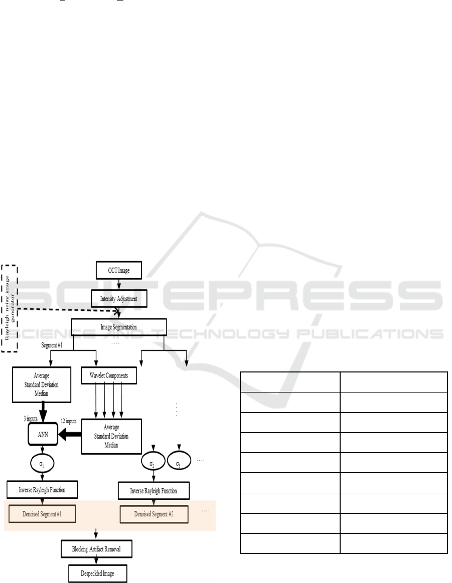
2.2 Speckle Reduction Algorithm

The algorithm we propose is composed of two phases.

The first phase is the training phase. Using a Rayleigh

noisy image generator in MATLAB, 10×10 pixels

images were generated with sigma values (the single

noise parameter employed in the Rayleigh function)

ranging from 0 to 255 in steps of 0.05. For each sigma

value, this procedure was repeated 100 times to

generate numerous noisy images for training.

Three features - average, standard deviation, and

median - were calculated from each segment and its

wavelet sub-bands for training. Wavelet sub-band

images were used to calculate the frequency domain

statistical knowledge of the image. The neural

network used is a combination of several MLP neural

networks. The flow chart of algorithm is given in

figure.2. Three MLP networks and a combiner, which

is responsible for the averaging process, are the main

components of this framework. Each of the MLP

networks is composed of 15 neurons in its input layer,

10 neurons in its hidden layer and one output neuron

to estimate the sigma parameter. The combiner is

responsible for averaging with L neurons in input

layer, L neurons in hidden layer and one output

neuron which can estimate the sigma parameter in an

ensemble fashion (in this paper, L = 3). To show the

advantage of ensemble method over individual neural

networks, let us consider a number of trained MLP

neural networks L with outputs 



 (where x is an

input vector). These estimate the sigma values using

the i

MLP neural network with an error of e

with

respect to the desired value of the sigma parameter,



. In this situation, the following equation can be

written as:









(1)

Thus the sum of squared error for the network y

can be calculated using eq. (2):



























(2)

where [.] denotes the expectation (average or

mean value). Thus the average error for the MLP

networks acting individually can be calculated by eq.

(3).







































(3)

By averaging the outputs 



, the committee

prediction is obtained. This estimate will have an

error equal to (eq. (4)):



















∑





















∑



















(4)

Thus, using the Cauchy’s inequality which is

shown in eq. (5), one can show that E

COM

≤ E

AV.

An Intelligent Speckle Reduction Algorithm for Optical Coherence Tomography Images





























1



























(5)

The neural network delivered the highest

reliability in the estimation of the sigma value when

a Daubechies 4 (db4) mother function was used.

There are a total of 12 inputs to the neural network.

The transfer function, performance function, learning

function, network size, and number of hidden layers,

were chosen experimentally such that optimum

network reliability is achieved. Such reliability is

defined as the percentage ratio of the difference

between the expected sigma value and the estimated

sigma over the expected sigma value. The averaged

reliability of the sigma estimator network measured

over 20 runs was 99.3 percent that was greater than

our previous ANN that had a reliability of 98.8

percent. The second phase is the testing phase. As

shown in the de-speckling flowchart in figure 2, the

OCT image is initially divided into several segments

based on the homogeneity. Similar to the training

stage, the same pre-processing was applied to each

image, and then the statistical features were extracted

Figure 2: Schematic diagram of the despeckling algorithm.

The blocks in the dotted box are used in the training phase.

from each segment in the image and used as input for

the neural network. The Rayleigh noise parameter

was then estimated for each segment using the trained

network (Avanaki and Hojjatoleslami, 2009). The

estimated sigma is then used along with a numerical

method to solve the inverse Rayleigh function

numerically for each segment. Putting together the

noise model segments, we can generate a noise model

image. The noise model image was deducted from the

original image with a scale factor which was obtained

experimentally. To remove the blocking artifact,

following the method given in (Fitzpatrick, 1975),

some statistical features were extracted from the

original image, based upon which of the despeckled

segments are then stitched together.

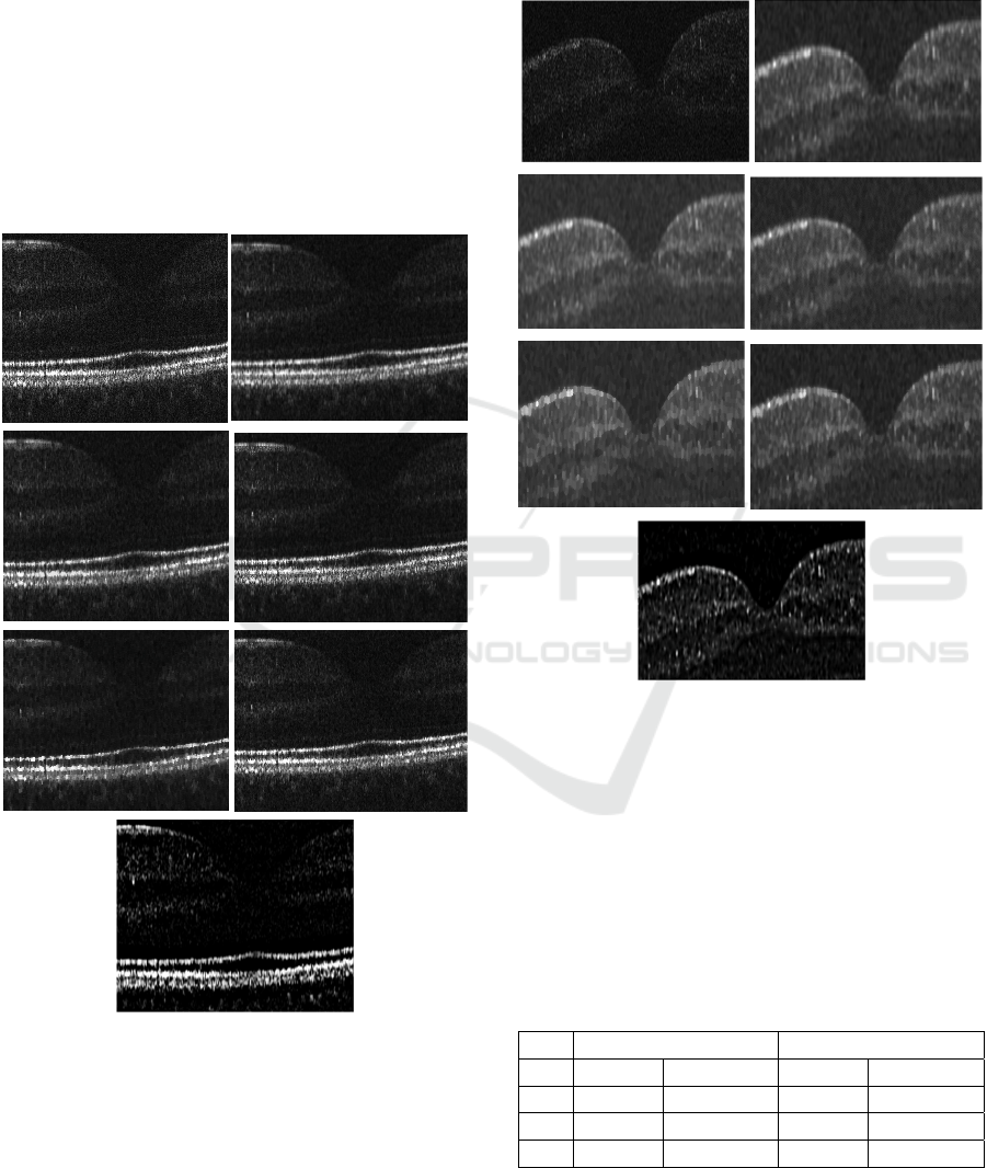
3 RESULTS AND DISCUSSION

B-scan OCT images of eye (in-vivo) were used to test

the algorithm. The OCT images before and after de-

speckling algorithm are shown in figure 3. The

number of segments in each image affects the

despeckling efficiency. To improve edge sharpness

and have more effective blocking artifact removal, we

segment our images into eight sub images. The

estimated sigma values for the segments within the

images are given in table 1, table 2 and table 3

corresponded to figure. 3, figure.4, figure.5

respectively.

Table 1: The estimated sigma values for figure. 3, The

number of segments are 8 (4 segments in each row).

Segment # Sigma

1 112

2 56

3 21

4 41

5 131

6 145

7 162

8 143

To evaluate the improvement of the images after

de-speckling, we calculated the signal-to-noise ratio

and the contrast-to-noise ratio (CNR) as defined in

eq. (6) and eq.(7) respectively (Shankar, 1986).

PHOTOPTICS 2016 - 4th International Conference on Photonics, Optics and Laser Technology

⎟

⎠

⎞

⎜

⎝

⎛

)(max

log10

SNR

(6)

⎟

⎠

⎞

⎜

⎝

⎛

−

∑

CNR

)(1

σσ

μμ

(7)

where max(I

) represents the maximum of

squared intensity pixel values in a homogeneous

region of interest in the linear magnitude image,

where

and

and CNR represents the mean,

variance of the same background noise region, and

and

represents the mean and variance of the R

region of interest (Shankar, 1986).

Table 2: The estimated sigma values for figure. 4, The

number of segments are 8 (4 segments in each row).

Segment # Sigma

1 98

2 64

3 51

4 45

5 68

6 20

7 39

8 81

Table 3: The estimated sigma values for figure. 5, The

number of segments are 8 (4 segments in each row).

Segment # Sigma

1 75

2 64

3 56

4 68

5 28

6 30

7 27

8 19

In-line with other published work (Shankar,

1986), we used 5 regions (R=5) in the calculation of

CNR. The results of these calculations on three test

images are given in Table 2. We compared the

performance of the proposed method in this article

with some other existing methods (see figure 3, figure

4 ad figure 5). We observed a blurring artifact in the

averaged image, as well as in the median filtered

image that was not observed in the denoised image

using our proposed method. It was also perceived that

the median filtered image is more pronounced in

terms of image contrast. The quantitative assessments

of the despeckled image showed in figure.3, figure.4

and figure.5 demonstrated that the proposed method

can provide an extra enhancement.

Figure 3: Comparative presentation of six despeckling

methods on an original OCT test images acquired from the

retina (optic nerve region) of a volunteer (AP), white male,

provided by Adrian Podoleanu’s lab. (a) Original B-scan

image of optic nerve, lateral size ~ 1-1.2 mm, (b) the B-scan

image after average filtering (window size: 3), (c) the B-

scan image after median filtering (window size: 3), (d), the

B-scan image after wiener filtering (window size: 3), (e) the

B-scan image after Kuwahara filtering (window size: 5), (f)

the B-scan image after SNN filtering (window size: 3), (g)

the B-scan image after using the proposed method.

(g)

(a)

(b)

(c)

(d)

(e)

(f)

An Intelligent Speckle Reduction Algorithm for Optical Coherence Tomography Images

of around 8 dB and 0.6 in terms of SNR and CNR

respectively compared to their counterparts in

averaging and median filtering Moreover, the

proposed method surpassed both Symmetric Nearest

Neighbourhood and Winner noise reduction filters by

increment of around 3dB in terms of SNR. However

in case of CNR a difference of 0.2 is observed.

Kuwahara filtered image has a SNR of 4dB and CNR

of 0.1 less than filtered image using proposed method

is depicted in figure.6. It should be noted that this fast

real-time effective algorithm could be enhanced by

utilizing a more accurate estimation of sigma

employing an improved version of ANN and using a

Figure 4: Comparative presentation of six despeckling

methods on an original OCT test images acquired from the

retina (optic nerve region) of a volunteer (AB-fovea), white

male (a) Original B-scan image of optic nerve,(b) the B-

scan image after average filtering (window size: 3), (c) the

B-scan image after median filtering (window size: 3), (d)

the B-scan image after wiener filtering (window size: 3), (e)

the B-scan image after Kuwahara filtering (window size: 5),

(f) the B-scan image after SNN filtering (window size: 3),

(g) the B-scan image after using the proposed method.

more precise valuation of noise model

mathematically. Moreover a possible improvement

can be achieved referring to image segments. A future

study planned to cover those issues.

Figure 5: Comparative presentation of six despeckling

methods on an original OCT test images acquired from the

retina (optic nerve region) of a volunteer (AB-fovea), white

male (a) Original B-scan image of optic nerve, (b) the B-

scan image after average filtering (window size: 3), (c) the

B-scan image after median filtering (window size: 3), (d)

the B-scan image after wiener filtering (window size: 3), (e)

the B-scan image after Kuwahara filtering (window size: 5),

(f) the B-scan image after SNN filtering (window size: 3),

(g) the B-scan image after using the proposed method. The

vertical axis is z-axis.

Table 4: Numerical assessment of the proposed denoising

algorithm using SNR and CNR metrics.

SNR CNR

Original Despeckled Original Despeckled

(I1) 9.2 26 2.5 4

(I2) 12.1 31 3 5.9

(I3) 11.5 24 1.9 3.2

(a) (b)

(c)

(d)

(e)

(f)

(g)

(a)

(b)

(e)

(f)

(g)

PHOTOPTICS 2016 - 4th International Conference on Photonics, Optics and Laser Technology

Figure 6: Comparative presentation of three original OCT

test images (I1), (I2), (I3) and of their denoised images.

4 CONCLUSIONS

In this paper, a speckle reduction algorithm was

presented based on the approximation that speckle

noise has a Rayleigh distribution with a noise

parameter, sigma. A new ensemble framework as a

combination of several Multi-Layer Perceptron

(MLP) neural networks was designed to estimate

sigma in the speckle noise model. The sigma

estimator kernel worked with more than 99.3%

reliability on average. The estimated sigma values

were then used in the de-speckling algorithm to

reduce the speckle in the OCT images. The algorithm

was successful in reducing speckle of B-scan images

of human eye. The algorithm reduced the speckle

while preserved the details of the regions. Two well-

established no-reference quality metrics including

SNR and CNR were used for quantitative evaluation,

and demonstrated higher quality images when the

new algorithm was utilized. The proposed algorithm

is also compared with some other bilateral digital

filters and demonstrated a satisfying evaluation.

Respectively, due to the generality of proposed ANN

algorithm, it can be used as a signal processing

method in other image modalities such as

photoacoustic imaging system (Nasiriavanaki et al.,

2014).

REFERENCES

Avanaki, M., Laissue, P. P., Eom, T. J., Podoleanu, A. G.

& Hojjatoleslami, A. 2013a. Speckle reduction using an

artificial neural network algorithm. Applied optics, 52,

5050-5057.

Avanki, M. R., Cernat, R., Tadrous, P. J., Tatla, T.,

Podoleanu, A. G. & Hojjatoleslami S. A. 2013b. Spatial

compounding algorithm for speckle reduction of

dynamic focus OCT images. Photonics Technology

Letters, IEEE, 25, 1439-1442.

Avanaki, M. R. & Hojjatoleslami, A. 2009. Speckle

reduction with attenuation compensation for skin OCT

images enhancement. Proceeding of Medical Image

Understanding and Analysis (MIUA), Kingston

University, London, 14-15.

Avanaki, M. R., Laissue, P. P., Podoleanu, A. G. & Hojat,

A. Denoising based on noise parameter estimation in

speckled OCT images using neural network. 1st

Canterbury Workshop and School in Optical Coherence

Tomography and Adaptive Optics, 2008. International

Society for Optics and Photonics, 71390E-71390E-9.

Fitzpatrick, T. B. 1975. Soleil et peau. J Med Esthet, 2, 33-

34.

Goodman, J. W. 2007. Speckle phenomena in optics: theory

and applications, Roberts and Company Publishers.

Nasiriavanaki, M.R.N, Xia, J., Wan, H., Bauer, A. Q.,

Culver, J. P. & Wang, L. V. 2014. High-resolution

photoacoustic tomography of resting-state functional

connectivity in the mouse brain. Proceedings of the

National Academy of Sciences, 111, 21-26.

Ozcan, A., Bilenca, A., Desjardins, A. E., Bouma, B. E. &

Tearney, G. J. 2007. Speckle reduction in optical

coherence tomography images using digital filtering.

JOSA A, 24, 1901-1910.

Podoleanu, A. G. 2014. Optical coherence tomography. The

British journal of radiology.

Shankar, P. M. 1986. Speckle reduction in ultrasound B-

scans using weighted averaging in spatial

compounding. IEEE transactions on ultrasonics,

ferroelectrics, and frequency control, 33, 754-758.

(I1)

(I2)

(I3)

An Intelligent Speckle Reduction Algorithm for Optical Coherence Tomography Images