Detecting People in Large Crowded Spaces using 3D Data from Multiple

Cameras

∗

ao Carvalho

, Manuel Marques

, Jo

ao Paulo Costeira

and Pedro Mendes Jorge

Institute for Systems and Robotics (ISR/IST), LARSyS, Instituto Superior T

ecnico, Univ. Lisboa, Lisbon, Portugal

ISEL - Instituto Polit

ecnico de Lisboa, Lisbon, Portugal

Keywords:

3D Point Cloud, Depth Camera, Multiple Cameras, Human Detection, Human Classiﬁcation.

Abstract:

Real time monitoring of large infrastructures has human detection as a core task. Since the people anonymity

is a hard constraint in these scenarios, video cameras can not be used. This paper presents a low cost solution

for real time people detection in large crowded environments using multiple depth cameras. In order to detect

people, binary classiﬁers (person/notperson) were proposed based on different sets of features. It is shown that

good classiﬁcation performance can be achieved choosing a small set of simple feature.

1 INTRODUCTION

Automatic human detection through 3D camera data

is a core problem in many contexts. Examples are

surveillance, human-robot interaction and human be-

haviour analysis. In this paper, it is proposed a

methodology with depth cameras for people detec-

tion in large crowded spaces while maintaining the

anonymity. The detection should be done in real time

and without using color information, in order to pre-

serve anonymity. These constraints are requested by

the real world scenario: the monitoring of waiting

queues and passages on an airport. Furthermore, the

characteristics of the areas to cover imply the use of

multiple depth cameras. The presented strategy seg-

ments candidates from the cameras data and classiﬁes

them into person or non-person. The procedure was

tested on a labelled dataset with several subsets of fea-

tures, in order to ﬁnd one that requires low computa-

tional effort while still achieving good results.

1.1 Related Work

Extensive literature is available regarding human de-

tection on RGB images (Moeslund et al., 2006). In

(Mikolajczyk et al., 2004), the authors propose a

method to detect people by using multiple body parts

∗

Carvalho, Marques and Costeira were supported by the

Portuguese Foundation for Science and Technology through

the project LARSyS - ISR [UID/EEA/50009/2013]. Jorge

was supported by SMART-er LISBOA-01-0202-FEDER-

021620/SMART-er/QREN.

detectors. A widely used approach to detect humans

in color images is to use the Histogram of Oriented

Gradients (HOG) descriptor (Dalal and Triggs, 2005).

To compute it, a given region of an image is divided

into a number of cells and for each cell the gradi-

ent of its pixels is computed. The resulting gradi-

ents are then integrated into a histogram. To avoid

the exhaustive process of sliding windows in search

of candidates, several methods have been proposed to

efﬁciently identify relevant regions of an image, such

as (Zhu et al., 2006). Stereo camera systems have

also allowed to achieve good results by estimating the

depth of the covered areas (Ess et al., 2009).To add

the three-dimensional information to video images,

the integration with laser range ﬁnders has been fre-

quently studied (Arras et al., 2007).

With the appearance of cheap depth cameras, such

as the Asus Xtion

, it became easy to merge color and

3D information in RGB-D images. Several methods

have been proposed to perform human detection with

such data. In (Spinello and Arras, 2011), the authors

propose the Histogram of Oriented Depth (HOD) de-

scriptor and combine it with the HOG descriptor, with

an approach that implies each frame to be exhaus-

tively scanned for people, implying a GPU implemen-

tation for real time usage. An alternative method is

proposed in (Mitzel and Leibe, 2011), where the peo-

ple detection is performed only in a set of regions of

interest (ROI). However, the process of ﬁnding these

http://www.asus.com/3D-Sensor/Xtion PRO/

speciﬁcations/

218

Carvalho, J., Marques, M., Costeira, J. and Jorge, P.

Detecting People in Large Crowded Spaces using 3D Data from Multiple Cameras.

DOI: 10.5220/0005727702180225

In Proceedings of the 11th Joint Conference on Computer Vision, Imaging and Computer Graphics Theory and Applications (VISIGRAPP 2016) - Volume 4: VISAPP, pages 218-225

ISBN: 978-989-758-175-5

regions requires a GPU implementation. In (Munaro

et al., 2012), it is proposed a fast solution to detect

people within groups using the depth data. The can-

didates found are ﬁltered by computing the HOG fea-

tures of the RGB region corresponding to the candi-

dates. A similar approach is proposed in (Liu et al.,

2015), where the segmentation is also done using the

3D data followed by classiﬁcation using a histogram

of height difference and a joint histogram of color and

height.

The methods referred all have the color informa-

tion as an important part of the detection or classi-

ﬁcation procedure. However, there are cases where

privacy and identity protection should be enforced.

In such cases, RGB cameras must be avoided to pre-

vent easy identiﬁcation of the subjects involved. Work

has been proposed that uses only the depth informa-

tion. In (Xia et al., 2011), a two-stage head detec-

tion process is employed, with a ﬁrst stage where a

2D edge detector ﬁnds a ﬁrst set of candidates in the

depth image, which are then selected using a 3D head

model. The contour of the body is then extracted

with a region growing algorithm. In (Bondi et al.,

2014), the heads are detected by applying edge detec-

tion techniques to the depth images. The heads detec-

tion can be also achieved in a probabilistic approach

(Lin et al., 2013). In (Hegger et al., 2013), the 3D

data is divided in several layers according to its height

and clustered using euclidean clustering. Each clus-

ter is then classiﬁed using the histogram of local sur-

face features and the clusters merged using connected

components, with a ﬁnal stage of classiﬁcation of the

merged clusters. In (Choi et al., 2013), the authors

present a method to segment the depth image using a

graph-based algorithm to determine ROIs. The HOD

descriptor is then computed for each ROI and classi-

ﬁed with a linear SVM. Other solution, (Brscic et al.,

2013), uses low cost depth cameras and high resolu-

tion laser range ﬁnders for large scale infrastructures.

1.2 Outline

The outline of the proposed method is presented on

Figure 1. The segmentation procedure is described in

Section 3. Section 4 presents the set of features ex-

tracted from each candidate. Afterwards, on Section

5, the classiﬁcation methods tested on this work are

presented. Section 6 presents the labelled dataset cre-

ated for this work. The results obtained are exposed

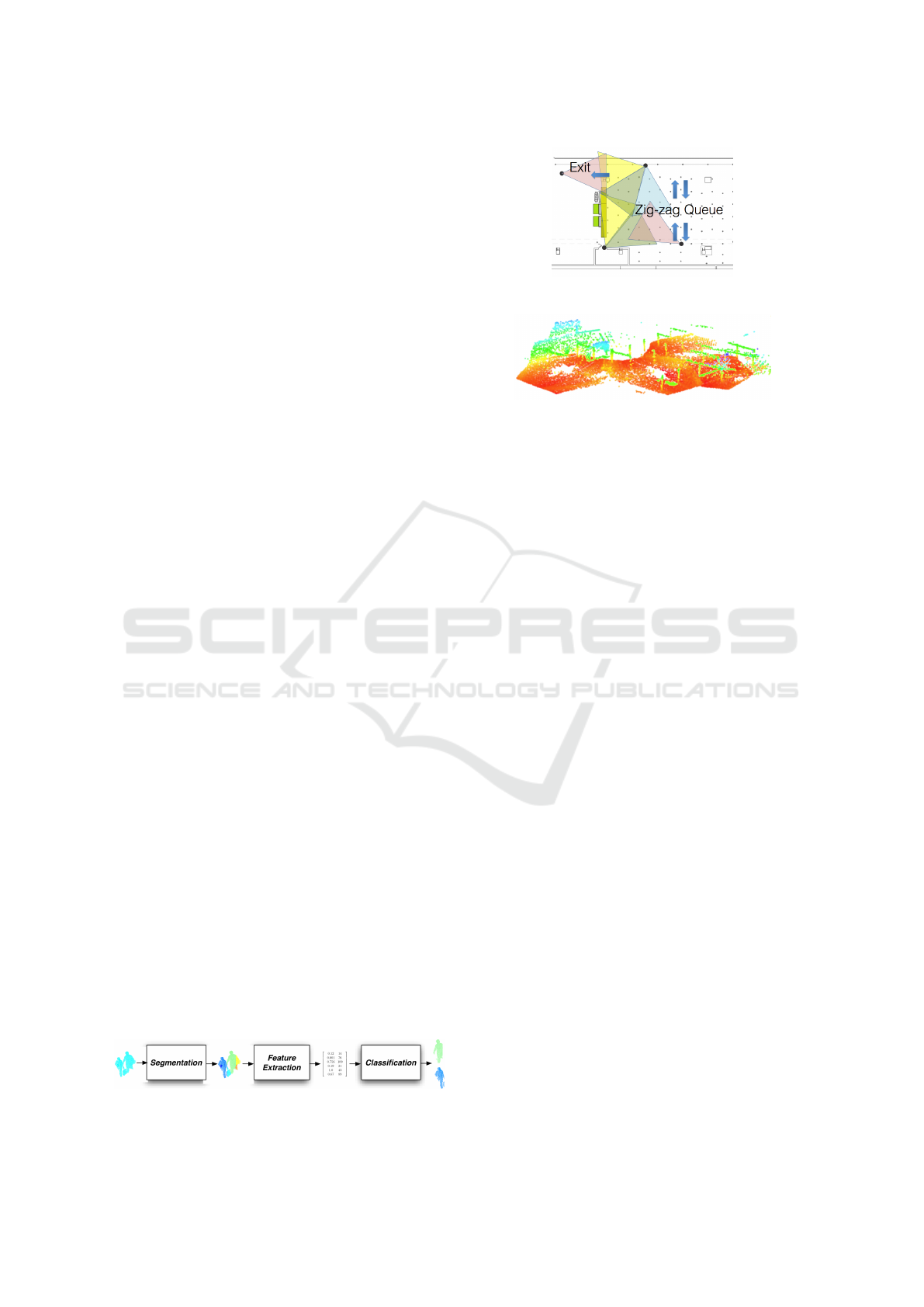
Figure 1: Methodology Outline. Three steps: segmentation,

feature extraction; classiﬁcation.

(a) Camera approximate setup

(b) A 3D point-cloud of the covered area

Figure 2: Waiting queue area camera setup: (a) approximate

camera locations and ﬁeld of view; (b) a 3D point-cloud of

the covered area.

on Section 7, followed by the future work and con-

clusions. Following, one presents the waiting queue

scenario, camera setup and its challenges.

2 REAL SCENARIO

CHALLENGES

To monitor the area of interest, one needs to com-

pute several metrics, some of which require the full

coverage of the space. Given the limited ﬁeld of

view (FOV) and range of depth cameras, this implies

the use of multiple cameras. However, although one

needs to completely cover the area, the overlap be-

tween cameras should be left to minimum, in order to

avoid the degradation of the data by the interference

of overlapping infrared patterns. Additionally, with

limited and low height locations to place the cameras,

several challenges are raised.

Figure 2(a) roughly illustrates the placement and

FOV of the depth cameras used to cover our real

world environment, a waiting queue area in a trans-

portation infrastructure. Figure 2(b) presents a point

cloud of the space captured without people. Note

the visible zig-zag queue guides. The cameras re-

quired accurate calibration to ensure that the transi-

tion of people from one camera to another would be

as “smooth” as possible. Very good intrinsic param-

eters are required to guarantee that the cameras re-

port the depth information as close as possible to the

true depth. Given a proper set of intrinsic parame-

ters, cameras require extrinsic calibration to ensure

that the relative pose of the cameras is as close as pos-

sible to the true value. However, even with a good

Detecting People in Large Crowded Spaces using 3D Data from Multiple Cameras

219

(a) Frontal view (b) Top view (c) Top view at

5.3m (data from

two cameras)

Figure 3: Point-cloud of a person: (a) frontal view (of points

with height above 1.30m) at about 3.3m from the camera;

(b) top view on the same location as in (a); (c) top view on

an area covered by two cameras, both at about 5.3m. The

data points of each camera are presented in different colors.

calibration, the point clouds from overlapping cam-

eras will never match perfectly, leading to much nois-

ier/fuzzier data. Additionally, the cameras used, Asus

Xtion PRO, have a maximum speciﬁed depth range

of 3.5m. In practice, however, to ensure full cover-

age, the depth data was used up to 5.5m. One should

note that as distance increases, the camera loses pre-

cision and the data becomes noisier. Moreover, the

ceiling of the area had a low height and the cam-

eras were ﬁxed at 2.3m from the ground. Having to

cover a distance of 5.5m from the mounting point,

this easily leads to severe occlusion of the people in

the queue. Figure 3(a) presents the point cloud of the

frontal view a person (only points with height above

1.30m) as viewed by a single camera at about 3.30m

from the camera. Figure 3(b) presents the same per-

son, at the exact same position but viewed from the

top. Finally, Figure 3(c) presents the point-cloud of

the same person from the top view on an area covered

by two cameras. The point-cloud is now much more

scattered and hardly (if) recognisable as a person pro-

ﬁle. Therefore, this setup leads to point clouds of very

occluded people or fuzzy point clouds.

3 DATA SEGMENTATION

This section presents the strategy used for the 3D

point cloud segmentation. This procedure was orig-

inally inspired by the method described in (Munaro

et al., 2012).

It should be noted that prior to the segmenta-

tion process, background subtraction is applied to the

depth images and the 3D data is transformed to the

global reference frame.

To illustrate the segmentation process, consider

the depth image in Figure 4(a) and the point cloud of

the closest foreground points, Figure 4(b). Having the

3D points in a global reference plane, the algorithm it-

eratively searches for the highest point and ﬁts a ﬁxed

sized box around that point. This encloses/clusters

(a) Depth image (b) Partial point cloud

Figure 4: Example of a depth image and partial point cloud:

(a) presents a depth image form the camera on exit 1; (b)

presents the point cloud of closest foreground points.

the surrounding points within the box. Afterwards,

the clustered points are removed from the cloud and

the procedure is iteratively repeated until no further

points are left to cluster. Figures 5(a) to 5(c) present

the ﬁrst three steps of the process and Figure 5(d)

presents the ﬁnal segmentation results, with one color

per cluster. The goal of iterating through points of

maximum height is that those points will be good can-

didates to “top of the head point” and a rough cen-

troid of a person. By using a ﬁxed size box, one is

assuming that a person occupies a maximum volume

and that people keep a certain minimum distance from

each other. In the presented example, despite success-

fully segmenting the two perceptible people (green

and bigger blue clusters), another four clusters are ex-

tracted. Therefore, a classiﬁcation strategy must be

used to ﬁlter the candidates.

Finally, note that while iterating through points of

maximum height, one only considers those points to

be a valid head point if it has a minimum number of

points bellow itself. This allows to further ﬁlter out

spurious high points that might degrade the segmen-

tation results.

Figure 6 presents a point cloud of the waiting

queue with several people and the result of applying

the segmentation procedure. Each cluster is displayed

with a unique color, although very similar colors ex-

ist.

4 FEATURE EXTRACTION

In order to successfully classify candidate clusters, a

set of relevant features must be extracted from the

point clouds. Having the requirement to segment and

classify dozens of point clouds in real-time, features

should be computationally light. Computation of nor-

mal vectors of points, principal component analysis,

(Hastie et al., 2009), or computationally demanding

procedures as such, can not be used.

The ﬁrst features to extract from a candidate point

cloud are the simplest features computed in this work:

VISAPP 2016 - International Conference on Computer Vision Theory and Applications

220

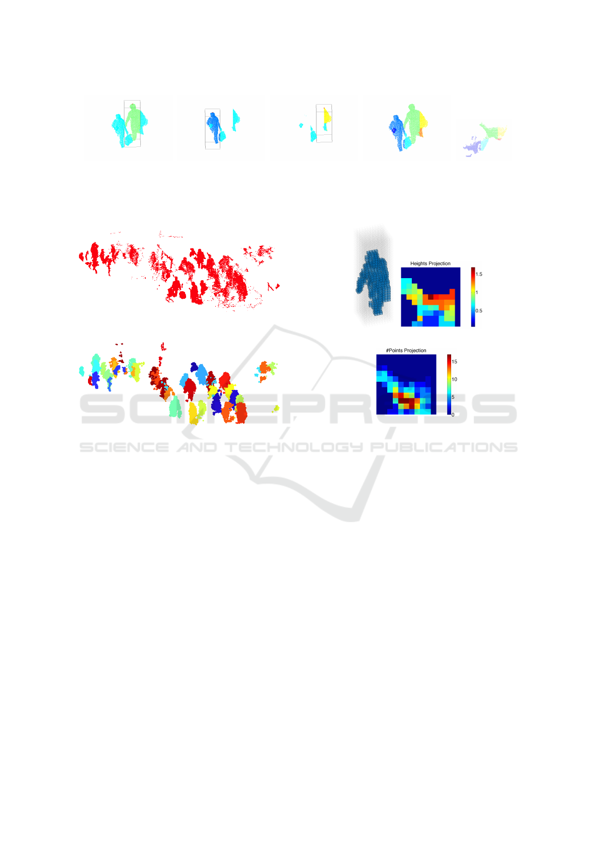
(a) Step 1 (b) Step 2 (c) Step 3 (d) Final (e) Final -

topview

Figure 5: Segmentation example: (a) to (c) frontal view of the ﬁrst three steps of the segmentation process with box and

highest point in red; (d) frontal view of the point cloud ﬁnal segmentation; (e) top view of the point cloud ﬁnal segmentation.

(a) Point cloud to segment

(b) Segmented point cloud

Figure 6: Example of the segmentation results for the wait-

ing queue point cloud: (a) point cloud prior to segmenta-

tion; (b) segmented point cloud, one color per cluster (very

similar colors exist).

the number of points of each cluster; the height of the

cloud, i.e., the height of the highest point; and the area

occupied by a cloud when its points are projected into

the ground. Following, to account for the shape of

the point cloud, a vector of features resulting directly

from the segmentation is built. This is what one de-

ﬁnes as voxels. For each segmented cluster, ﬁt a ﬁxed

size box, centered exactly on its highest point. Af-

terwards, the box is divided by a regular grid, where

each cell of that grid, a voxel, is set to one if at least

one data point is in it and zero otherwise. For this

work, the box has dimensions 0.66m ∗0.66m ∗2.1m.

Figure 7(a) presents an example of a voxelized point

cloud with a voxel matrix of 11 ∗11 ∗35, i.e., with

0.06m size voxel. This grid of voxels is then vector-

ized and used as feature vector.

Other features to be used are the ground projec-

tion of the heights and the ground projection of the

number of points. Both projections are represented

by a 11 ∗11 matrix, dimensions equal to the ﬁrst two

(a) (b)

(c)

Figure 7: Feature examples: (a) voxels; (b) heights projec-

tion on the ground; (c) number of points projection on the

ground.

dimensions of the voxel grid. The number of points

(in fact, number of voxels) projection is the sum of

the voxel cells along the third dimension of the grid

(recall that voxel cells have 0/1 value). Figure 7(c)

presents such a matrix. On the heights projection,

each cell of the matrix contains the height of the high-

est point falling into that cell, Figure 7(b). Similarly,

to the voxels, these matrix are vectorized to be used

as feature vector.

Finally, a more complex descritor is computed,

the Ensemble of Shape Functions (ESF), proposed

in (Wohlkinger and Vincze, 2011). It considers dis-

tances between pairs of sampled points, angles be-

tween lines formed by three sampled points and areas

of triangles built using randomly sampled points.

In summary, the full set of features is:

• number of points;

• height;

• area;

• heights projection;

• number of points

projection;

• voxels;

• ESF.

Detecting People in Large Crowded Spaces using 3D Data from Multiple Cameras

221

5 CLASSIFICATION METHODS

This section presents the two classiﬁers tested for this

human detection procedure, the Support Vector Ma-

chine (SVM), (Cortes and Vapnik, 1995), and the

Random Forest (RF), (Breiman, 2001).

5.1 Support Vector Machine

A support vector classiﬁer is a binary classiﬁcation

method that computes a hyperplane to separate obser-

vation points from two distinct classes. The goal is to

ﬁnd the hyperplane to which the distance between the

observation points and the hyperplane is maximum.

The computation of this hyperplane is done by solv-

ing the optimization problem

max

,β,ε

,...,ε

s.t. y

(β

+ β

) ≥ M(1 −ε

)

||β|| = 1

≥ 0

∑

i=1

≤C,

for all i ∈ {1,...,N}. M is the separating margin, ε

are the slack variables and C is a non-negative con-

stant. By forcing the last constraint, one is impos-

ing a bound on the margin and hyperplane violations.

Therefore, if C = 0 no margin violation is allowed.

When C is small, the margin is small and rarely vio-

lated. When C is large, the margin is wider and more

violations are allowed. The C parameter is normally

chosen through cross-validation (CV).

On this work, besides the linear classiﬁcation on

the original feature space, one also maps the features

to a higher-dimensional space by using a SVM with a

gaussian kernel:

K(x, ˜x) = exp



−γ||x − ˜x||



For further information on SVM, refer to (Cortes and

Vapnik, 1995) and (Hastie et al., 2009).

5.2 Random Forests

Random forests is a method based on decision trees,

(Breiman, 2001). Decision trees are capable of cap-

turing complex structures in data and have relatively

low bias. However, they are noisy, suffering from

high variance. Random forests improve decision trees

by reducing their variance and consequently decreas-

ing their error rate. This is achieved by decreasing

the correlation between trees, training each tree with

(a) (b) (c)

Figure 8: Example of an observation per person class: (a)

complete person observation, sideways, with backpack; (b)

waist up person observation, frontal view; (c) shoulders up

person observation, slightly sideways.

different subset of the data points and by randomly

selecting a subset of features at each node split.

RF allow the estimation the generalization error

without using CV. The observations not used in the

training of a tree are called out-of-bag (OOB) obser-

vations. For each point in the dataset, one can select

the trees in which the point was OOB and get the clas-

siﬁcation of that point for each of those trees and get

a ﬁnal result through majority vote. The OOB classi-

ﬁcation error can be computed by applying this pro-

cedure to every point on the dataset. It can be shown

that the OOB error is equivalent to the leave-one-out

cross-validation error for sufﬁciently large number of

trees.

Another interesting characteristic of the RF is the

capability of assessing feature importance. After the

RF training, to compute the importance of a particu-

lar feature, one randomly permutes the values of that

feature across the OOB points and recomputes the er-

ror. The diference in the classiﬁcation accuracy from

the original OOB points and the permuted ones gives

a measure of importance of the feature.

For further information on RF, refer to (Breiman,

2001) and (Hastie et al., 2009).

6 DATASET LABELLING

A dataset was built for this work by manually la-

belling segmented point clouds. To perform the la-

belling, the data was visually inspected. The raw data

of the dataset, acquired at an airport, consists of im-

ages from eight depth cameras. Seven from the area

presented on Figure 2 and an additional one from a

close area. The 3D point clouds were computed from

these images, segmented and merged on a global ref-

erence frame. Although the point clouds could have

been labelled separately for each camera, the intent

was to use the data as it was used on the referred

project, with overlapping areas.

Although in this work only two classes are con-

VISAPP 2016 - International Conference on Computer Vision Theory and Applications

222

sidered for classiﬁcation, person or non-person, the

point clouds were labelled in four classes: complete

person, waist up person, shoulders up person and non-

person. The reason is that there exists frequent oc-

clusion when the space is crowded, and by labelling

people depending on their visibility one can more eas-

ily inspect classiﬁcation results and hopefully under-

stand better in which cases the classiﬁer fails. Fig-

ure 8 presents and observation from each of the per-

son classes. Please note that for training the classi-

ﬁers, these three classes were merge into a unique

one. Note also that the dataset is noisy. People can

be observed from several views, from the front, from

the back, sideways or something in-between. Also, as

previously referred, the point clouds get noisier with

the distance from the cameras as on the areas where

the data from multiple cameras overlap.

A total of 1345 point clouds were labelled, with

542 non-people, 545 complete body people, 183 waist

up people and 75 shoulders up people.

7 EXPERIMENTAL RESULTS

As referred in the previous section, the three person

classes were merged into a unique one. To balance the

dataset, the observations corresponding to complete

body people were down sampled such that the total

number of person observations matches the number

of non-people.

From this dataset, the features described in Sec-

tion 4 were computed and applied standardization to

all of them. Also, features with null standard devia-

tion (features equal for all points on the dataset) were

removed. With these features, several subsets were

built to train the classiﬁers:

• f1: {heights, number of points, areas} ∈ R

;

• f2: {heights projection} ∈ R

121

;

• f3: {number of points projection} ∈ R

121

;

• f4: {f1, f2, f3} ∈ R

245

;

• f5: {voxels} ∈ R

3390

;

• f6: {ESF} ∈ R

612

;

• f7: {f4, f5, f6} ∈ R

4247

The purpose of this feature separation into several

subsets is to assess their performance versus all the

features, f7. For each subset, training was done for a

SVM with linear kernel, a SVM with gaussian kernel

and a random forest.

For training and validation purposes, the dataset

was divided into training and test data, with 759 ob-

servations (∼ 70%) and 325 observations, respec-

Table 1: Training CV error rates for the linear SVM

(LSVM), gaussian SVM (GSVM) and OOB error rate for

the RF. The subset of features to which the classiﬁer had

lower error is in bold type.

CV Error OOB Error

LSVM GSVM RF

f1 0.0501 0.0408 0.0461

f2 0.0514 0.0435 0.0422

f3 0.0988 0.0738 0.0646

f4 0.0277 0.0303 0.0343

f5 0.0382 0.0290 0.0343

f6 0.0856 0.0896 0.0725

f7 0.0264 0.0290 0.0369

Table 2: Classiﬁcation error rates for the training and test

datasets. The subset of features to which the classiﬁer had

lower error is in bold type. The lowest error for the test

dataset is underlined.

Test Data Error

LSVM GSVM RF

f1 0.0554 0.0554 0.0400

f2 0.1077 0.0923 0.0585

f3 0.1015 0.0677 0.0554

f4 0.0462 0.0523 0.0338

f5 0.0400 0.0400 0.0400

f6 0.0831 0.0862 0.0492

f7 0.0431 0.0277 0.0246

tively. The SVMs were trained with 5-fold cross-

validation in order to compute the best parame-

ters for the classiﬁer. For the linear kernel, one

tested a total of 20 logarithmically spaced values

of C ∈ [10

−5

,10

]. For the gaussian kernel, one

tested 10 values for C ∈ [10

−2

,10

] and 10 values for

γ ∈ [10

−6

,10

]. The parameters with lowest cross-

validation error were chosen as the best ones and used

to evaluate the model on the test dataset. The random

forest was trained with 250 decision trees and

√

p fea-

tures chosen at each node split.

For testing the SVM classiﬁers, one used the

MATLAB toolkit PMTK3

. For building the RFs, it

was used the Statistics and Machine Learning Tool-

box for MATLAB. All the features were implemented

in MATLAB, with the exception for the ESF. The ESF

is implemented in the PCL library (Rusu and Cousins,

2011).

Table 1 reports, for all feature sets, the CV error

of each SVM “winning” model and the OOB error

for the RF with 250 trees. The linear SVM (LSVM)

achieves the lowest CV error, 0.0264, when using all

the features, f7, but obtains a very close error for f4.

For the gaussian SVM (GSVM), the best training re-

https://github.com/probml/pmtk3 - PMTK3 webpage.

Last accessed on August 26, 2015.

Detecting People in Large Crowded Spaces using 3D Data from Multiple Cameras

223

sults are obtained for f5 and f7, with 0.0290 of error.

For the random forests (RF), the lowest OOB error

is obtained for f4 and f5, with 0.0343, but with close

results for f7.

Table 2 presents the classiﬁcation error rate of

each classiﬁer and set of features for the test obser-

vations. The three classiﬁers had the exact same er-

ror rate for f4, however, for all the other subsets the

RF outperformed the SVM classiﬁers. The best re-

sult was obtained using f7, with a 0.0246 error rate.

The LSVM performed best for f4, with 0.0400 error

rate, and the GSVM for f7, close to the RF result, with

0.0277.

Besides the lower error for the test dataset, the RF

classiﬁer has the advantage of being simple to train

and not prone to overﬁtting (James et al., 2013). With

RFs, assuming m =

√

p as proposed by the authors,

one only has to choose the number of trees to train.

On the other hand, with the SVM, one has to choose

a kernel, choose a range of values for the classiﬁer

and kernel parameters and use cross-validation to ﬁnd

the best values. Depending on the kernel used and

number of parameter values tested, this can lead to

long training times. For instance, with f7, the training

of the RF took 14.13s of cpu time, while the SVMs

took 83.18s and 1743.22s for the linear and gaussian

kernels, respectively.

While training the RF for the f7 feature set, the

OOB feature importance was recorded. The three

simplest features, i.e., heights, number of points and

areas, are exactly the features with higher importance,

with 1, 0.9115 and 0.9119, respectively

. One should

note that this tool evaluates the importance of each

feature space dimension individually and that only

these ﬁrst three dimensions can be seen as individ-

ual. All the other dimensions of the space are part of

“composed” features, such as the voxels or the ESF.

So, even if the most important features are the three

referred, the composed features end up having more

importance when all of its dimensions are summed.

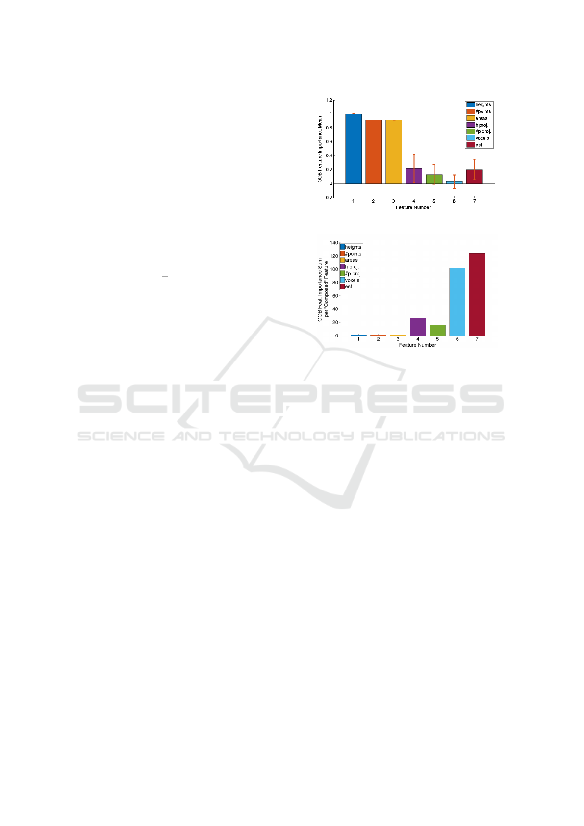
Figure 9(b) presents the sum of feature importance

by composed feature. One can see that the composed

feature that has higher “summed” oob importance is

the ESF. This comes a litle surprising as the ESF (f6)

is far from being the best feature subset according to

Table 2. From this one can conclude that even if the

sum of the importante of a composed feature is much

higher than some other feature, that does not neces-

sarilly mean that the composed feature will lead to

lower error rates. Figure 9(a) presents the mean of

the OOB feature importance for each composed fea-

ture. One can easilly understand that if one is to use

a small number of features, the heights, the number

Values normalized by the maximum importance value.

(a)

(b)

Figure 9: OBB Feature importance: (a) mean per “com-

posed” feature set; (b) summed per “composed” feature set.

of points and the area are the ones to use. The voxels

have the lowest mean, as many of its cells have neg-

ative importance, meaning they lead to the decrease

of the accuracy. There are also zero importance cells,

cells that made no difference in the classiﬁcation or

were never tested for node splitting.

The testing data set was formed by 159 non-

person observations, 91 complete body observations,

53 waist up observations and 22 shoulders up obser-

vations. For each of these subclasses, the best LSVM

misclassiﬁed 4.40%, 4.40%, 3.77% and 0%, respec-

tively. The GSVM misclassiﬁed 3.77%, 1.10%,

3.77% and 0%. The RF misclassiﬁed 2.52%, 3.30%,

1.89% and 0%. These results show that, contrary to

what could be expected, the classiﬁers do not present

signiﬁcant differences in misclassiﬁcation percentage

between the point clouds corresponding to occluded

and non-occluded people. Further, the observations

from people visible only from the shoulders up were

all correctly classiﬁed.

To achieve real time performance, the segmen-

tation and feature extraction procedures were im-

plemented in C. The candidates are classiﬁed by a

Python RF implementation (Pedregosa et al., 2011).

The segmentation and classiﬁcation procedures take

around 0.2ms per person, for the f1. It must be

noted that the segmentation implementation is not op-

timized and further improvements can be achieved.

VISAPP 2016 - International Conference on Computer Vision Theory and Applications

224

8 CONCLUSIONS

This paper presented a low-cost solution for human

detection in large infrastructures while preserving

people identity. Real time performance is achieved by

using a small set of simple features. It was presented

a real scenario in which multiple depth cameras are

simultaneously used to monitor the environment. The

method uses the merged data from the cameras and

ﬁnds candidates by segmenting the resulting 3D point

cloud. For each candidate, a set of features is ex-

tracted. Several subsets of features were tested to as-

sess their performance when used as input to a classi-

ﬁer. The proposed classiﬁer lies on features with low

computational cost and achieves good performance in

a real time scenario.

As future work, it would be interesting to explore the

creation of conﬁdence regions on the FOV of each

camera to account for the accuracy degradation with

the distance.

ACKNOWLEDGEMENTS

The authors would like to thank Jo

ao Mira, Thales

Portugal S.A. and ANA Aeroportos de Portugal for

enabling the data acquisition within the SMART-er

project and Susana Brand

ao by providing the ESF

MATLAB wrapper.

REFERENCES

Arras, K. O., Mozos,

O. M., and Burgard, W. (2007). Us-

ing boosted features for the detection of people in 2d

range data. In IEEE ICRA, pages 3402–3407. IEEE.

Bondi, E., Seidenari, L., Bagdanov, A. D., and Del Bimbo,

A. (2014). Real-time people counting from depth im-

agery of crowded environments. In Advanced Video

and Signal Based Surveillance (AVSS), 11th IEEE In-

ternational Conference on, pages 337–342. IEEE.

Breiman, L. (2001). Random forests. Machine learning,

45(1):5–32.

Brscic, D., Kanda, T., Ikeda, T., and Miyashita, T. (2013).

Person tracking in large public spaces using 3-d range

sensors. Human-Machine Systems, IEEE Transac-

tions on, 43(6):522–534.

Choi, B., Meric¸li, C., Biswas, J., and Veloso, M. (2013).

Fast human detection for indoor mobile robots us-

ing depth images. In IEEE ICRA, pages 1108–1113.

IEEE.

Cortes, C. and Vapnik, V. (1995). Support-vector networks.

Machine learning, 20(3):273–297.

Dalal, N. and Triggs, B. (2005). Histograms of oriented

gradients for human detection. In IEEE CVPR Com-

puter Society Conference on, volume 1, pages 886–

893. IEEE.

Ess, A., Leibe, B., Schindler, K., and Van Gool, L. (2009).

Moving obstacle detection in highly dynamic scenes.

In IEEE ICRA, pages 56–63. IEEE.

Hastie, T., Tibshirani, R., and Friedman, J. (2009). The

elements of statistical learning.

Hegger, F., Hochgeschwender, N., Kraetzschmar, G. K.,

and Ploeger, P. G. (2013). People detection in 3d

point clouds using local surface normals. In RoboCup

2012: Robot Soccer World Cup XVI, pages 154–165.

Springer.

James, G., Witten, D., Hastie, T., and Tibshirani, R. (2013).

An introduction to statistical learning. Springer.

Lin, W.-C., Sun, S.-W., and Cheng, W.-H. (2013). Demo

paper: A depth-based crowded heads detection sys-

tem through a freely-located camera. In IEEE ICME

Workshops, pages 1–2. IEEE.

Liu, J., Liu, Y., Zhang, G., Zhu, P., and Chen, Y. Q. (2015).

Detecting and tracking people in real time with rgb-d

camera. Pattern Recognition Letters, 53:16–23.

Mikolajczyk, K., Schmid, C., and Zisserman, A. (2004).

Human detection based on a probabilistic assembly

of robust part detectors. In Computer Vision-ECCV,

pages 69–82. Springer.

Mitzel, D. and Leibe, B. (2011). Real-time multi-person

tracking with detector assisted structure propagation.

In IEEE ICCV Workshops, pages 974–981. IEEE.

Moeslund, T. B., Hilton, A., and Kr

uger, V. (2006). A sur-

vey of advances in vision-based human motion cap-

ture and analysis. Computer vision and image under-

standing, 104(2):90–126.

Munaro, M., Basso, F., and Menegatti, E. (2012). Tracking

people within groups with rgb-d data. In IEEE/RSJ

IROS International Conference on, pages 2101–2107.

IEEE.

Pedregosa, F., Varoquaux, G., Gramfort, A., Michel, V.,

Thirion, B., Grisel, O., Blondel, M., Prettenhofer,

P., Weiss, R., Dubourg, V., Vanderplas, J., Passos,

A., Cournapeau, D., Brucher, M., Perrot, M., and

Duchesnay, E. (2011). Scikit-learn: Machine learning

in Python. Journal of Machine Learning Research,

12:2825–2830.

Rusu, R. B. and Cousins, S. (2011). 3D is here: Point Cloud

Library (PCL). In IEEE ICRA, Shanghai, China.

Spinello, L. and Arras, K. O. (2011). People detection in

rgb-d data. In IEEE/RSJ IROS International Confer-

ence on, pages 3838–3843. IEEE.

Wohlkinger, W. and Vincze, M. (2011). Ensemble of shape

functions for 3d object classiﬁcation. In IEEE RO-

BIO International Conference on, pages 2987–2992.

IEEE.

Xia, L., Chen, C.-C., and Aggarwal, J. K. (2011). Human

detection using depth information by kinect. In IEEE

CVPR Workshops Computer Society Conference on,

pages 15–22. IEEE.

Zhu, Q., Yeh, M.-C., Cheng, K.-T., and Avidan, S. (2006).

Fast human detection using a cascade of histograms of

oriented gradients. In IEEE CVPR Computer Society

Conference on, volume 2, pages 1491–1498. IEEE.

Detecting People in Large Crowded Spaces using 3D Data from Multiple Cameras

225