
Monocular Depth Ordering using Perceptual Occlusion Cues
Babak Rezaeirowshan, Coloma Ballester and Gloria Haro
Department of Information and Communication Technologies, Universitat Pompeu Fabra, Barcelona, Spain
Keywords:
Monocular Depth, Ordinal Depth, Depth Layering, Occlusion Reasoning, Convexity, T-junctions, Boundary
Ownership, 2.1D.
Abstract:
In this paper we propose a method to estimate a global depth order between the objects of a scene using
information from a single image coming from an uncalibrated camera. The method we present stems from
early vision cues such as occlusion and convexity and uses them to infer both a local and a global depth
order. Monocular occlusion cues, namely, T-junctions and convexities, contain information suggesting a local
depth order between neighbouring objects. A combination of these cues is more suitable, because, while
information conveyed by T-junctions is perceptually stronger, they are not as prevalent as convexity cues in
natural images. We propose a novel convexity detector that also establishes a local depth order. The partial
order is extracted in T-junctions by using a curvature-based multi-scale feature.Finally, a global depth order,
i.e., a full order of all shapes that is as consistent as possible with the computed partial orders that can tolerate
conflicting partial orders is computed. An integration scheme based on a Markov chain approximation of the
rank aggregation problem is used for this purpose. The experiments conducted show that the proposed method
compares favorably with the state of the art.
1 INTRODUCTION
Depth perception in humans enables a robust 3D vi-
sion even in the presence of a single view stimulus.
Such a system is desirable in computer vision mainly
due to its many applications and the abundance of
monocular cameras. Human vision harnesses monoc-
ular cues to resolve inherent ambiguity caused by 3D
to 2D projection in the image formation process and
creates a sensible 3D perception. Monocular depth
perception cues consist of dynamic cues and static
cues. Dynamic cues, such as motion occlusion and
motion parallax require multiple frames and motions
in the scene as stimuli which are out of scope of this
work. In this proposal, the focus is on static cues,
namely, convexity and T-junctions; other cues in this
category are perspective, relative dimensions, lighting
and shadow.
While physiological aspects of these cues have
been widely studied in the literature of psychophysics
and vision, there is only a handful of research works
that test these theories in a practical scenario using
computer vision methods. Most of the work related to
depth estimation in computer vision focuses on stereo
disparity or motion parallax, both of which use tri-
angulation to compute depth. While triangulation-
based methods provide absolute depth, which is de-
sirable in many applications, they require two or more
views. Monocular static cues on the other hand, can
be combined to create a depth perception in the ab-
sence of binocular and dynamic monocular cues or as
a complement to improve existing depth perception in
a much wider domain.
The goal of this paper is, given a single image
from an uncalibrated camera and its decomposition
in shapes (that are assumed to represent the projec-
tion of the 3D objects on the image plane; e.g., a seg-
mentation), to create a globally consistent depth order
of these shapes that constitute the image scene. For
this purpose, occlusion cues between objects, namely
T-junctions and convexities are used. Following the
underlying assumption for extracting depth from oc-
clusion cues, we assume that the image is composed
of objects that are fronto-parallel to the camera. This
is also referred to as the dead leaves model, a term
coined by Matheron (Matheron, 1968), which consti-
tutes a model for image formation where the image is
made by objects falling on top of each others and par-
tially occluding them. The reason for making such as-
sumption is that in the presence of non fronto-parallel
objects in the image, e.g. floor, occlusion does not
translate to depth order (see Figure 1).
Given an image that satisfies the dead leaves
model, the occlusion cues provide a depth order
Rezaeirowshan, B., Ballester, C. and Haro, G.
Monocular Depth Ordering using Perceptual Occlusion Cues.
DOI: 10.5220/0005726404310441
In Proceedings of the 11th Joint Conference on Computer Vision, Imaging and Computer Graphics Theory and Applications (VISIGRAPP 2016) - Volume 4: VISAPP, pages 431-441
ISBN: 978-989-758-175-5
Copyright
c
2016 by SCITEPRESS – Science and Technology Publications, Lda. All rights reserved
431

Figure 1: Dead leaves model (DLM) and correctness of
convexity cues. The left image follows the DLM while the
right one doesn’t. Arrows indicate the occluding object sug-
gested by convexity cues. Bright arrows indicate a correct
depth order while dark arrows indicate a wrong one.
among neighbouring regions. However, we require
a global order to establish a rough 3D model of the
scene, which is understood here as obtaining a con-
sistent global order from a number of partial orders,
which may contain some discrepancies. This problem
is in general referred to as rank aggregation and it has
been dealt with in several fields of computer science
(Dwork et al., 2001; Basha et al., 2012). This ordering
problem appears whenever there are multiple opera-
tors providing partial orders with transitive relations.
The goal is to use the transitivity to obtain a global
robust order as consistent as possible with the partial
orders. Transitivity between orders can be stated as
the following property: if we have a partial order in-
dicating A<B and another one indicating B<C, thus
we can infer the global order A<B<C. Our approach
stems from the fact that transitivity of local orders can
be utilized to obtain a global order using rank aggre-
gation.
Our main contributions in this paper are (i) a depth
ordering system based on monocular perceptual cues
that allows reasoning without need for camera cali-
bration, multiple frames, or motion, (ii) a novel gen-
eral convexity cue detector that assigns a local depth
order based on convexity and which is based on the
convex hull of a shape, and (iii) the extraction of a
global depth order by a robust integration of the par-
tial orders.
2 RELATED WORK
3D modeling has received a significant attention from
the computer vision community, with studies focus-
ing on various aspects of 3D perception. Due to the
vastness of the literature in this field, we will focus
on studies conducted on monocular static cues. Com-
putational methods for depth extraction from a sin-
gle image can be categorized into supervised methods
and Gestalt-based methods. Supervised methods ei-
ther learn depth directly from training images (Saxena
et al., 2008; Eigen et al., 2014), or alternatively learn
and detect cues (Chen et al., 2013; Jia et al., 2012),
geometric (Hoiem et al., 2011) or semantic (Liu et al.,
2010) information and use them to infer an abso-
lute depth. Aforementioned approaches are aimed
at a specific type of scene (either outdoor or indoor
scenes) and require additional training or parameter
tuning to achieve high performance on the unfamil-
iar scenes. Alternatively, other approaches have been
suggested in the literature that use human perception
and vision as the basis from which to attempt to infer a
computational model simulating the known processes
of human vision. Our work falls in the latter category.
Thus, we focus on the use of T-junctions and convex-
ity cues for establishing a depth order. The role of T-
junctions as a cue for recovering surface occlusion ge-
ometry was introduced by (Guzm
´
an, 1968), and later
stressed by (Malik, 1987; Rubin, 2001). Moreover,
through the Gestalt school of thought in psychology,
T-junctions were described as a basis of monocular
depth perception by the work of Kanizsa (Kanizsa,
1979). Later on, more computational works demon-
strated the capability of T-junctions for depth estima-
tion; to the best of our knowledge, one of the first
attempts at depth ordering methods using T-junctions
was performed by (Marr, 1982). Later on, an inspiring
work of Nitzberg et al. (Nitzberg and Mumford, 1990;
Nitzberg et al., 1993) proposed the so-called 2.1D
sketch through a joint segmentation and depth esti-
mation model. More recently, studies have been con-
ducted using energy minimization approaches which
use either explicit (Gao et al., 2007; Palou and Salem-
bier, 2011) or implicit (Esedoglu and March, 2003)
junction detection algorithms.
In addition to T-junctions, convexity is consid-
ered to be one of the most dominant cues for figure-
ground organization (Kanizsa, 1979). A computa-
tional model for utilizing convexity has been devel-
oped for figure-ground organization in the recent past
(Pao et al., 1999). Moreover, works on occlusion rea-
soning using Gestalt-based methods have used con-
vexity as a complementary cue to T-junctions for
a more robust relative depth estimation (Dimiccoli
et al., 2008; Calderero and Caselles, 2013; Palou
and Salembier, 2013). While it has been suggested
that convexity affects human depth perception and is
coded explicitly in the brain (Burge et al., 2010), the
literature in computational models that use convex-
ity is divided in this sense. In the works (Dimiccoli
et al., 2008; Palou and Salembier, 2013), convexity
is explicitly detected and coded, while in (Calderero
and Caselles, 2013) this is done implicitly. The pro-
posed approach shares with (Dimiccoli et al., 2008;
VISAPP 2016 - International Conference on Computer Vision Theory and Applications
432
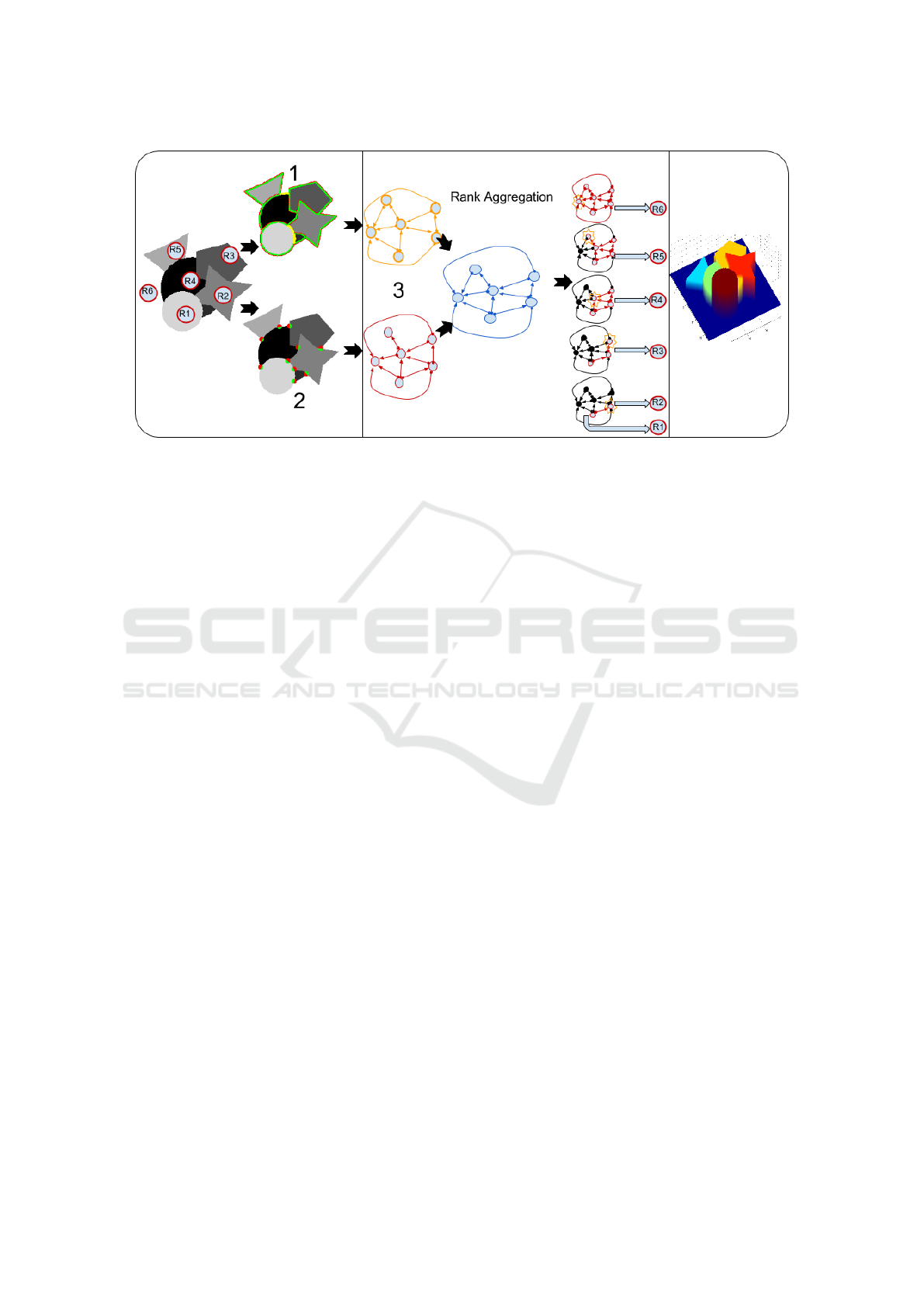
Figure 2: Diagram of the proposed method. From left to right: The segmented image; detected convexities cues (above) and
T-junctions cues (below) and the local depth order from each cue inferred by the local cues (green areas are in front of red
ones, whereas yellow indicates an inconclusive cue); global depth order extraction by rank aggregation on a graph whose
nodes represent the different shapes and the directed edges indicate local depth orders; final result with global depth order
illustrated as a depth map, where warmer color values indicate closer objects to the camera.
Palou and Salembier, 2013; Calderero and Caselles,
2013) the use of convexity and T-junctions cues. In
order to integrate the partial depth orders suggested
by the monocular depth cues we use a graph-based
approach. Previous works (Dimiccoli and Salembier,
2009b; Palou and Salembier, 2013) also use a graph
representation but need to reduce it to an acyclic graph
and remove conflicts among different cues. In con-
trast, our work can directly handle conflicting transi-
tive orders in the graph by using a rank-aggregation-
based method (Basha et al., 2012), and obtain a glob-
ally consistent depth order. Here, transitive order is
the order established by a path in the graph involv-
ing more than two nodes using the transitivity prop-
erty mentioned in Section 1. A very recent work on
depth layering using occlusion cues is the work of
(Zeng et al., 2015) where convexity, T-junctions and a
ground contact cue is used to obtain a depth order of
the image. An energy minimization scheme is used to
find the correct depth order which makes their method
more complex and time consuming than our proposed
method. Moreover, they have to make more restric-
tive assumptions to obtain the correct ground contact
cue which limits their method to a smaller domain.
As the method proposed by (Zeng et al., 2015) shows
promising results and performs superior to other sim-
ilar methods (Jia et al., 2012; Palou and Salembier,
2013), it has been used as a benchmark for evaluation
of our proposed method. A comparative evaluation
using the experimental setup in (Zeng et al., 2015) is
presented in Section 4.
3 PROPOSED METHOD
We propose a method to extract a global depth or-
der from a single image from an uncalibrated cam-
era. The idea is motivated by studies showing human
vision capability to integrate monocular depth cues to
create a sensible depth perception. Given an input im-
age, let us consider the set of its (segmented) shapes -
the notion of shape used in this paper will be clarified
in Section 3.1.1. Then, a global depth order can be
obtained following the steps below:
1. Determine a local depth order between each pair
of adjacent shapes by analysing the convexity of
their common boundaries.
2. Detect T-junctions and use a multi-scale feature to
determine a local depth order between the shapes
that meet at each T-junction.
3. Establish a global depth order by rank aggregation
of the previous partial local orders.
Each step of the proposed method is detailed in the
following sections. Figure 2 illustrates the different
steps of the algorithm.
3.1 Local Depth Cues Detection
Local depth cues are extracted to establish a local
depth order between neighbouring objects. In this
work, convexities (L-junctions) and T-junctions are
used for this purpose. We use a segmentation of
Monocular Depth Ordering using Perceptual Occlusion Cues
433

the image as an input to the cue detection mecha-
nism. In order to compute a local depth order in a
manner that follows the human perception based on
psychophysics studies (Kanizsa, 1979; McDermott,
2004; Burge et al., 2010), T-junctions and convexi-
ties must be treated in a different manner. Thus, an
explicit detection of such depth cues is required. In
the following, we explain how we detect both kind of
junctions.
3.1.1 Convexity Cue
In this paper we propose a global convexity decision
about each connected boundary between any two ad-
jacent (segmented) regions in the image. The aim of
this step is to determine which side of the boundary is
the occluder and which side is the occluded, thus es-
tablishing a local depth order. Given the dead leaves
model assumption, this cue can be used to infer the
local depth order of the shapes that share a boundary.
To find the occluding region, we propose a method
to determine which side of the boundary is closer to
a convex shape. Figure 3 illustrates this process. Ini-
tially the segmented image is used to obtain the set
of all the common boundaries between any two re-
gions or objects in the image (Fig. 3, left image). For
each connected common boundary, we consider its
bounding box (shown in Fig. 3, middle-up). A con-
nected common boundary divides the bounding box
into two shapes (denoted by S and S
0
in Fig. 3). The
shape whose area is closer to the area of its convex
hull (i.e. smaller red area in Fig. 3, middle-down) is
considered more convex and assigned as the occluder
(S in the example of Fig. 3). On the other hand, the
complement shape (S
0
in Fig. 3) is assigned as the oc-
cluded.
Let us notice that there is the possibility that a
given boundary does not provide a conclusive depth
cue. In other words, the convexity cue does not pro-
vide enough information to clarify which side is the
occluder and which side is the occluded. This phe-
nomenon appears, for instance, when the common
boundary is either a straight line or a sinusoidal curve.
To deal with such cases we define a criteria based on
Figure 3: Illustration of the main steps of the convexity cue
detector and the estimated local order where green areas are
estimated to be in front of red areas.
a threshold on our proposed global convexity measure
of the connected boundary between two adjacent re-
gions. This criteria is derived from the absolute dif-
ference between the convexity defect areas (red areas
in Fig. 3) of the shapes (S and S
0
). If this value is not
significant enough (i.e. it is lower than a prescribed
threshold thr
CX
) then these boundaries are considered
inconclusive and will have no effect on the result. We
define this threshold as thr
CX
= L · π · thr, where L is
the length of the boundary and thr is a tuning param-
eter that controls the sensitivity of the criteria and is
independent of the length of the boundary. Examples
of such inconclusive boundaries for different values
of thr can be found in Figure 4; namely, the figure dis-
plays examples for a smaller value of thr = 0.0 and a
bigger value of thr = 0.6. In order to study the effect
of this parameter, both on the local and global depth
ordering, we present in Section 4 some experiments
where the threshold thr is modified in the range of
[0.0, 0.6] with step size of 0.05.
Figure 4: Illustration of modifying the value of thr
CX
through the parameter thr. Top row, thr = 0.5; bottom row,
thr = 0.15. Decreasing thr leads to accepting more conclu-
sive boundaries (less inconclusive boundaries in yellow).
3.1.2 T-junctions Cue
One of the pivotal depth cues used in this paper are
T-junctions. T-junctions appear at the meeting points
of three shapes boundaries and are related to occlu-
sion configurations (see Figure 2). Two of the three
regions present in the T-junction are separated by the
stem of the T; these two regions are perceived to be
partly occluded by the region which presents a larger
section or angle. The latter region is then in front
of the other two. Moreover, the angle of each object
forming the junction must satisfy some criteria to be
classified as a T-junction.
In this paper, we compute T-junctions using the
method in (Caselles et al., 1999) where the authors
gave a definition of T-junction which overcomes the
difficulty of computing angles in a discrete image.
VISAPP 2016 - International Conference on Computer Vision Theory and Applications
434
They proposed an efficient algorithm which is mainly
based on thresholding and computes junctions di-
rectly on the image without previous preprocessing
or smoothing. The segmented image is used as an in-
put to this method and the output is the locations of
T-junctions.
The definition is based on the topographic map of
an image u : Ω ∈ R
2
→ R (in our case, the segmented
image), that is, the family of the connected compo-
nents of the so-called, level sets of u, [u ≥ λ] := {x ∈
Ω : u(x) ≥ λ}, and on its boundaries, the so-called
level lines. Here, λ represents the gray level of the
segmented image u. The set of level sets is invariant
to monotonic non-decreasing illumination changes, a
classical requirement in image processing and com-
puter vision (Serra, 1986), and the level lines contain
the boundaries of the parts of the physical objects pro-
jected on the image plane.In practice, the algorithm
computes the T-junctions as all the pixels p where
two level lines meet and such that the area of the con-
nected component of each of the bi-level sets [u ≤ α],
[α < u < β], [u ≥ β], with α < β, meeting at p is big
enough.
After detecting the location of T-junctions, for es-
tablishing a local depth ordering one could use some
angle or area of the regions meeting at the T-junction,
both of which have been used in the literature (Dim-
iccoli and Salembier, 2009a; Palou and Salembier,
2013). Problems arise when certain configurations of
the cue lead to an inaccurate computation. One of the
problems is related to the scale at which the depth cue
is obtained.
Noise in the image can also lead to incorrect cues,
so one could use larger scales but they are less dis-
criminative in depth. To avoid these issues, we stem
from the work by (Calderero and Caselles, 2013) to
create a reliable multi-scale measure to establish a lo-
cal depth order (according to human vision) at the lo-
cated cues. To this end, features are formulated using
the curvature of the level lines of the distance func-
tion of each connected component in the segmented
image at different scales. The features are computed
for each scale s by adding the contribution from each
connected component using the following formula:
E
s
(x) =
nc
∑
c=1
(e
β
s
|
K
c,s
(x)
|
γ
s
− 1), (1)
where K
c,s
is the curvature of the level lines of the dis-
tance function to the connected component c at scale
s, nc is the number of connected components at scale
s, γ
s
and β
s
are scale-related parameters which are
fixed as proposed in (Calderero and Caselles, 2013).
In order to keep these features local and avoid over-
lapping with other boundaries, the distance function
is clipped at a distance 5. In order to generate a multi-
scale local feature we combine the local features ac-
cording to (1) by computing an average of the nor-
malized features at several scales, as in (Calderero
and Caselles, 2013). In this work, we integrate the
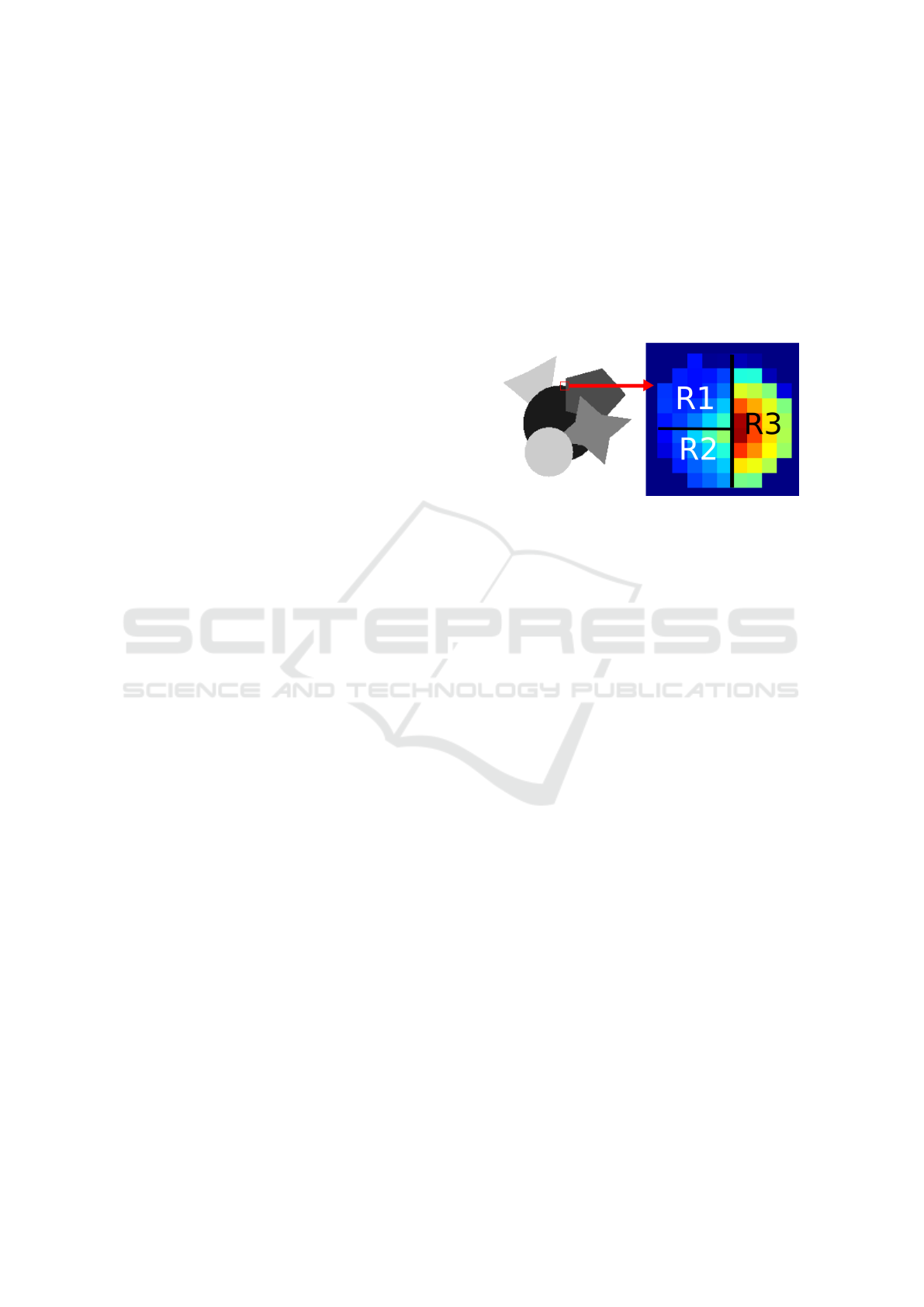
features from scales 1 to 5. Figure 5 illustrates with
an example the behaviour of this multi-scale features.
As it can be seen in Fig. 5 right, the part of the cue
that is perceptually closer to the observer has a higher
multi-scale feature value.
Figure 5: Multi-scale features obtained after averaging the
features E
s
(1) of the first five scales.
Finally, to estimate the local depth order induced
by a certain T-junction, first a representative value of
the multi-scale depth features is computed for each re-
gion (e.g. R1, R2, and R3 in Fig. 5 right) in the neigh-
borhood of the T-junction given by a disk of radius
5. The representative value is computed by applying
either the median or max operators on the features of
the respective region (i.e. R1, R2, R3). In section 4
we compare the performance of both operators. The
region with a higher representative local feature value
is assigned to be in front of the other two neighboring
regions (R3 in front of R1 and R2 in the example of
Fig. 5).
3.2 From Local to Global Depth
In order to establish a global depth order given by the
local cues we use an approximation of rank aggre-
gation (Dwork et al., 2001) similar to the one used
in (Basha et al., 2012) for photo-sequencing. To do
so, we construct a weighted graph G(U, E) to rep-
resent the partial order between pairs of shapes (ob-
jects), which are represented in the graph by the nodes
in U . The graph is constructed by placing a direc-
tional edge e(i, j) ∈ E connecting the node i to node j
if the local cues relating the objects suggest that object
i is in front of object j (represented here by i >> j).
The weight of the edge gathers up the local depth or-
der cues. Each convexity cue indicates a depth order
relation between two nodes (e.g. i << j) and each T-
junctions indicates a relation between three nodes us-
ing two edges (e.g. i << j, i << k). The weight of
Monocular Depth Ordering using Perceptual Occlusion Cues
435

Figure 6: Experiments with synthetic images: estimated global depth ordering (brighter gray levels indicate closer objects).
The automatically detected local depth cues, convexities and T-junctions establish a local depth order (green areas are esti-
mated to be in front of red areas). Inconclusive convexity cues are marked in yellow.
the edge e(i, j) between nodes i and j is proportional
to the number of local cues indicating the local order
i >> j, which can be interpreted as proportional to
the number of votes for the local order i >> j. This
weight corresponds to the probability that i >> j. In
such a graph, a random walk after a sufficient time (in
the steady state) will reach the sink of the graph (or of
a sub-graph) which represents the object (or objects)
perceptually furthest from the viewer. Repeating this
process iteratively while in each iteration removing
the sink node (or nodes) from the previous iteration
will provide us with the global depth order. In par-
ticular the iteration number in which a set of nodes is
removed reveals the global order of this set of nodes.
For illustration of this process see Figure 2- step 3.
The steady state can be computed using an eigen-
vector analysis of M, the transition state matrix asso-
ciated to the graph. The elements of M are the proba-
bilities of moving from one state (node) to another. To
construct the matrix M with non-negative entries, we
initially form a matrix V collecting the votes, where
the rows and columns indices correspond to the index
of each associated connected component. Thus, an
image with N shapes will produce an N × N matrix
V . The i, j-th element of matrix V , V (i, j), collects
the number of votes (local cues) that agree with the
partial ordering i >> j.
Once the matrix V is filled, we compute the matrix
M which specifies the probability that i >> j. Firstly,
the cycles of length two which may have been intro-
duced by conflicting cues are removed. We follow the
method proposed in (Basha et al., 2012) to resolve
these conflicts. In particular, M(i, j) = 1 −
V ( j,i)
V (i, j)
, and
M( j, i) = 0 if V (i, j) > V ( j, i). The rest of the cycles
do not need to be removed since the rank aggregation
method automatically solves them. Finally, the rows
of M are normalized to 1 in order to get transition
probabilities.
4 EXPERIMENTAL RESULTS
This section presents three different experiments with
different kind of data designed to evaluate and illus-
trate various aspects of the proposed method. An ini-
tial experiment is first presented as a proof of concept
using synthetic images with the following parameters:
thr = 0.15 for convexity cue detection, and median
as T-junction feature operator. The goal of the sec-
ond experiment is twofold: first, to present an exper-
imental study of different parameter settings to find
the best performance and fix the parameter values for
the rest of the experiments and, second, to provide a
quantitative comparison of the proposed method and
the most recent state-of-the-art methods (Jia et al.,
2012; Palou and Salembier, 2013; Zeng et al., 2015).
This experiment is done using a dataset of 52 images
proposed by (Zeng et al., 2015). For both the first
and second experiments the ground truth segmenta-
tion is available, whereas in the third experiment the
segmentation is done using an interactive tool (Sant-
ner et al., 2010).
Figure 6 illustrates the results of applying the pro-
posed method to a small set of synthetic images. The
first row shows the input images and the second row
shows the global depth order images with convexity
and T-junctions cues superimposed on them, respec-
tively. The local depth order is illustrated in each
cue, where green indicates the section perceived to
be closer to the observer. As for global depth or-
der, the grey values indicate global depth order, par-
ticularly the brighter areas are closer to the observer.
As it can be seen all T-junction cues indicate a cor-
rect local depth order, whereas some of the convexity
VISAPP 2016 - International Conference on Computer Vision Theory and Applications
436
0 0.1 0.2 0.3 0.4 0.5 0.6
0.5
0.55
0.6
0.65
0.7
0.75
0.8
0.85
0.9
0.95
thr
CX
Accuracy adj. pairs
Med TJ + CX + GRA
Max TJ + CX + GRA
CX + GRA
CX No GRA
Med TJ + GRA
Max TJ + GRA
Figure 7: Accuracy of local depth order between adjacent
pairs of shapes.
0 0.1 0.2 0.3 0.4 0.5 0.6
0.54
0.56
0.58
0.6
0.62
0.64
0.66
0.68
0.7
thr
CX
Accuracy all pairs
Med TJ + CX + GRA
Max TJ + CX + GRA
CX + GRA
Med TJ + GRA
Max TJ + GRA
Figure 8: Accuracy of global depth order between all pairs
of shapes.
Table 1: Depth Order accuracy.
adj.
pairs
all
pairs
(Jia et al., 2012) 79.84 29.88
(Palou and Salembier, 2013) 43.85 43.56
(Zeng et al., 2015) 82.66 84.60
Our method: CX+GRA 74.83 59.21
Our method: TJ+GRA 84.39 65.3
Our method: TJ+CX+GRA 91.49 69.94
cues are incorrect or inconclusive (marked as yellow).
However, the T-junctions cues are able to compensate
these errors and create a globally consistent depth or-
der that complies with human depth perception.
In the first part of the second experiment the pro-
posed method is evaluated under different parameter
settings with the dataset proposed by (Zeng et al.,
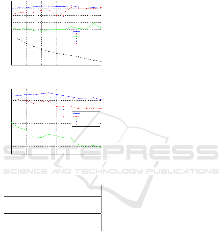
2015). Figures 7 and 8 illustrate these results. The
horizontal axis denotes the parameter thr that defines
the threshold thr
CX
= L · π · thr applied to the differ-
ence of defect areas. Then, as the values in the hori-
zontal axis increase the threshold thr
CX
increases and
more boundaries become inconclusive, meaning that
the sensitivity for detecting global convex boundaries
decreases (see also Fig. 4). In Figure 7 the vertical
axis indicates the accuracy as the percentage of pairs
of adjacent shapes which have been assigned a cor-
rect local depth order. Whereas in Figure 8 the ver-
tical axis indicates the accuracy as the percentage of
pairs of all shapes which have been assigned a cor-
rect global depth order. These accuracy measures are
identical to the measures of performance evaluation
in (Zeng et al., 2015). The legend of Figures 7 and
8 indicate the operator for the T-junction (median or
max), the type of local cue (T-junction (TJ), convex-
ity (CX) or both), and whether or not a global rank
aggregation was used (”GRA” or ”No GRA”). Both
Figures 7 and 8 indicate that the best performance
is achieved when the depth order induced by the T-
junction cues is computed using the median opera-
tor and is combined with the depth order induced by
the convexity cue using rank aggregation, denoted as
”Med T J +CX +GRA”. Thus, achieving a top perfor-
mance of 91.49% accuracy in local depth order esti-
mation and 69.94% in global depth order estimation.
On the other hand, using the max operator slightly
decreases the performance to 89% and 67.8% for lo-
cal and global depth estimation, respectively.The de-
crease in accuracy of the global order with respect
to the local order can be explained by the fact that
the proposed method can only infer depth relations
between objects connected by a path in the graph.
It should also be noted that the performance of the
max operator is slightly less stable. Further, it can
be seen that the contribution of T-junctions is signif-
icant for both global and local depth estimation as
they improve the performance compared to when only
convexities are used (16% increase for local depth
estimation and 19% increase in accuracy of global
depth estimation). The blue and red stars in the Fig-
ures 7 and 8 highlight the performance of using only
T-junctions (the parameter thr does not affect this
computation). As expected, T-junctions seem to be a
more reliable cue than convexities as they consistently
achieve a higher accuracy. Figure 7 illustrates how
the global integration of convexity cues using rank
aggregation improves the performance of local depth
estimation between adjacent pairs of shapes, namely,
the performance increases from 59% to 75%. Finally,
observing the two lower curves the in Figure 7 we
can see that, while the accuracy of ”CX + No GRA”
decreases as the threshold increases, the accuracy of
”CX +GRA” remains relatively stable. This indicates
that most of the convexity cues in the dataset are con-
clusive (i.e. comply with human depth perception)
and increasing the threshold will lead to less cues and
thus less accuracy. However, it is interesting to note
Monocular Depth Ordering using Perceptual Occlusion Cues
437

Figure 9: Depth ordering results using the proposed method on near-view scenes from the dataset by (Zeng et al., 2015).
that the global integration is able to compensate for
the removal of cues that did not satisfy the threshold
and stabilize the performance.It can be seen that the
best operation point for the threshold of the global
convexity is the mid-range value thr = 0.25, where
the average of the two accuracy measures is the high-
est. While the effect of thr is not significant it leads
to a slight increase in the performance of the global
depth estimation (see Figure 8).
In the second part of the second experiment, the
proposed method is compared with the state-of-the-
art (Jia et al., 2012; Palou and Salembier, 2013; Zeng
et al., 2015) with the accuracy measures presented in
(Zeng et al., 2015). According to the results obtained
in the previous analysis, we fix the parameters to the
following values: thr = 0.25 and median as the opera-
tor in the depth order estimated from the T-junctions.
To this end, we follow the experimental setup sug-
gested by (Zeng et al., 2015) on their proposed depth
ordering dataset. The results in Table 1 show that us-
ing a combination of T-junction and convexity cues
achieves the highest performance. As it can be seen,
the proposed method outperforms all of the state-of-
the-art methods in the adjacent pairs case and, in the
all pairs case, the proposed method performs superior
to (Jia et al., 2012) and (Palou and Salembier, 2013)
but falls short of (Zeng et al., 2015). This is mainly,as
previously noticed, due to the fact that our proposed
method cannot infer depth relations between objects
that are not are not connected with a path in our graph
i.e. there are no transitive relations to be used to infer
a global depth order. In contrast, the method by (Zeng
et al., 2015) uses the ground contact as an extra cue
to order shapes when other cues (T-junction, convex-
ity) are not present. This could be added in order to
make the constructed graph more connected. In other
words there are more transitive relations (paths) that
can be used to infer depth relations. All the previ-
ous experiments were carried out using Matlab on an
eight core 3.5GHz Core i7 processor with an average
computation time of 8.4 seconds per image.
Finally, to show how the proposed method may be
used as a real world application, the interactive seg-
mentation tool (Santner et al., 2010) has been used
to segment some images from the Berkeley dataset
(Martin et al., 2001) and the global depth order of
the segmented objects is estimated with the proposed
method. As it can be seen in Figure 10 the order of
the segmented objects is correct in most of the cases.
VISAPP 2016 - International Conference on Computer Vision Theory and Applications
438

Figure 10: Using interactive segmentation (Santner et al., 2010) and the proposed method to create a depth ordering of objects
in the scene.
5 LIMITATIONS AND
ASSUMPTIONS
Estimating depth from a single image is a very chal-
lenging and under-determined problem. It is neces-
sary to make suitable assumptions to make the prob-
lem tractable. Our first assumption is that a good
segmentation is available where the boundaries of the
segmentation regions coincide with the actual object
boundaries. As the method is based on a convexity
cue defined on boundaries and T-junctions (which are
points at the intersection of boundaries), a deficient
segmentation leads to significant depth artifacts in the
estimated depth order. A second limitation may be
noticed in one of the examples in Figure 11: the one
in box 1 of the left image. The T-junction and con-
vexity cues that are detected on the ground contact
of the object indicate incorrect depth order. In some
cases, there exist other cues that compensate for these
mistakes, either directly or indirectly using the transi-
tivity property of the graph. However, this is not the
case in the aforementioned example. Another limita-
tion is inaccuracies in our convexity detector which
can be seen in Figure 11 box 2, a misinterpretation of
convexities in cases where a long narrow shape is next
to two concavities. Figure 11 box 3 shows the bias of
the proposed method to interpret small convex objects
to be in front of their neighbouring shapes (this may
happen also in visual holes, such as windows or arch
bridges). A more general limitation is that objects in
the scene should be approximated with fronto-parallel
planes to the camera. When this assumption does not
hold it may lead to misinterpretation of local cues and
thus misestimation in the order of objects. An exam-
ple of this can be found in Fig. 11 right, box 4. In this
case, since the two objects sharing the same border
cannot be approximated with fronto-parallel planes,
the algorithm misestimates the depth order. Fortu-
nately, in some cases there are solutions to deal with
the aforementioned limitations. The non-fronto par-
allel problem can be resolved by ground separation
in simple cases. In cases where there are more than
one non-fronto parallel planes in the image, a geo-
metric context method, based for instance on surface
normal extraction, may be used to guide the depth es-
timation. The problem related to visual holes can be
addressed using a semantic labelling method that is
able to identify the visual hole; for example by classi-
fying areas like the sky which are always in the back.
6 DISCUSSION AND
CONCLUSION
Inspired by the human vision capability to perceive
depth using monocular cues, we proposed a method
for the detection and integration of T-junction and
convexity cues that is able to obtain a globally con-
sistent depth order. The proposed method computes
partial depth orders using multi-scale features, then,
integrates them using a rank aggregation method that
resolves conflict. This allows to simultaneously com-
pensate for incorrect partial depth orders introduced
by invalid cues and also harnesses the transitivity be-
tween the cues to obtain a global order from partial or-
ders. The proposed method is applicable to any scene
that complies with the dead leaves model and does
not require training. For future work we propose to
extend the method to images containing non fronto-
parallel objects using other monocular and binocular
cues that may be integrated in the rank aggregation
step as additional votes for partial depth orders.
ACKNOWLEDGEMENTS
The authors acknowledge partial support by MICINN
project, reference MTM2012-30772, and by GRC ref-
erence 2014 SGR 1301, Generalitat de Catalunya.
Monocular Depth Ordering using Perceptual Occlusion Cues
439

Ground
Truth
Estimated
Depth order
Original
Images
1
2
3
4
Figure 11: Due to some limitations of the proposed approach, the violation of certain assumptions leads to errors in the
estimated depth order which have been delimited with red boxes (see Section 5 for a detailed explanation of these problems).
REFERENCES
Basha, T., Moses, Y., and Avidan, S. (2012). Photo sequenc-
ing. In Computer Vision–ECCV 2012, pages 654–667.
Springer.
Burge, J., Fowlkes, C., and Banks, M. (2010). Natural-
scene statistics predict how the figure–ground cue of
convexity affects human depth perception. The Jour-
nal of Neuroscience, 30(21):7269–7280.
Calderero, F. and Caselles, V. (2013). Recovering Relative
Depth from Low-Level Features Without Explicit T-
junction Detection and Interpretation. International
Journal of Computer Vision, 104:38–68.
Caselles, V., Coll, B., and Morel, J. (1999). Topographic
maps and local contrast changes in natural images. In-
ternational Journal of Computer Vision, 33(1):5–27.
Chen, X., Li, Q., Zhao, D., and Zhao, Q. (2013). Occlusion
cues for image scene layering. Computer Vision and
Image Understanding, 117(1):42–55.
Dimiccoli, M., Morel, J.-M., and Salembier, P. (2008).
Monocular depth by nonlinear diffusion. In Com-
puter Vision, Graphics & Image Processing, 2008.
ICVGIP’08. Sixth Indian Conference on, pages 95–
102. IEEE.
Dimiccoli, M. and Salembier, P. (2009a). Exploiting
t-junctions for depth segregation in single images.
Acoustics, Speech and Signal . . . , pages 1229–1232.
Dimiccoli, M. and Salembier, P. (2009b). Hierarchical
VISAPP 2016 - International Conference on Computer Vision Theory and Applications
440

region-based representation for segmentation and fil-
tering with depth in single images. Image Processing
(ICIP), 2009 16th, 1:3533–3536.
Dwork, C., Kumar, R., Naor, M., and Sivakumar, D. (2001).
Rank aggregation methods for the web. In Proceed-
ings of the 10th international conference on World
Wide Web, pages 613–622. ACM.
Eigen, D., Puhrsch, C., and Fergus, R. (2014). Depth map
prediction from a single image using a multi-scale
deep network. In Advances in Neural Information
Processing Systems, pages 2366–2374.
Esedoglu, S. and March, R. (2003). Segmentation with
depth but without detecting junctions. Journal of
Mathematical Imaging and Vision, 18(1):7–15.
Gao, R., Wu, T., Zhu, S., and Sang, N. (2007). Bayesian
inference for layer representation with mixed markov
random field. Energy Minimization Methods in Com-
puter Vision and Pattern Recognition, 4679:213–224.
Guzm
´
an, A. (1968). Decomposition of a visual scene into
three-dimensional bodies. In Proceedings of the De-
cember 9-11, 1968, fall joint computer conference,
part I, pages 291–304. ACM.
Hoiem, D., Efros, A., and Hebert, M. (2011). Recovering
Occlusion Boundaries from an Image. International
Journal of Computer Vision, 91(3):328–346.
Jia, Z., Gallagher, A., Chang, Y., and Chen, T. (2012).
A learning-based framework for depth ordering. In
Computer Vision and Pattern Recognition (CVPR),
2012 IEEE Conference on, pages 294–301. IEEE.
Kanizsa, G. (1979). Organization in vision: essays on
Gestalt perception. NY, Praeger.
Liu, B., Gould, S., and Koller, D. (2010). Single image
depth estimation from predicted semantic labels. In
Computer Vision and Pattern Recognition (CVPR),
2010 IEEE Conference on, pages 1253–1260. IEEE.
Malik, J. (1987). Interpreting line drawings of curved
objects. International Journal of Computer Vision,
73403.
Marr, D. (1982). Vision: A computational approach. San
Francisco: Free-man & Co.
Martin, D., Fowlkes, C., Tal, D., and Malik, J. (2001).
A database of human segmented natural images and
its application to evaluating segmentation algorithms
and measuring ecological statistics. In Proc. 8th Int’l
Conf. Computer Vision, volume 2, pages 416–423.
Matheron, G. (1968). Mod
`
ele s
´
equentiel de partition
al
´
eatoire. Technical report, CMM.
McDermott, J. (2004). Psychophysics with junctions in real
images. Perception, 33(9):1101–1127.
Nitzberg, M. and Mumford, D. (1990). The 2.1-d sketch.
In Computer Vision, 1990. Proceedings, Third Inter-
national Conference on, pages 138–144. IEEE.
Nitzberg, M., Mumford, D., and Shiota, T. (1993). Filter-
ing, segmentation, and depth, volume 662. Lecture
notes in computer science, Springer.
Palou, G. and Salembier, P. (2011). Occlusion-based depth
ordering on monocular images with binary partition
tree. In Acoustics, Speech and Signal Processing
(ICASSP), 2011 IEEE International Conference on,
pages 1093–1096. IEEE.
Palou, G. and Salembier, P. (2013). Monocular depth or-
dering using t-junctions and convexity occlusion cues.
IEEE Transactions on Image Processing, 22(5):1926–
1939.
Pao, H., Geiger, D., and Rubin, N. (1999). Measuring con-
vexity for figure/ground separation. In Computer Vi-
sion, 1999. The Proceedings of the Seventh IEEE In-
ternational Conference on, volume 2, pages 948–955.
IEEE.
Rubin, N. (2001). Figure and ground in the brain. Nature
Neuroscience, 4:857–858.
Santner, J., Pock, T., and Bischof, H. (2010). Interactive
multi-label segmentation. In Proceedings 10th Asian
Conference on Computer Vision (ACCV), Queen-
stown, New Zealand.
Saxena, A., Chung, S. H., and Ng, A. Y. (2008). 3-d depth
reconstruction from a single still image. International
journal of computer vision, 76(1):53–69.
Serra, J. (1986). Introduction to mathematical morphology,
volume 35(3). Elsevier.
Zeng, Q., Chen, W., Wang, H., Tu, C., Cohen-Or, D.,
Lischinski, D., and Chen, B. (2015). Hallucinating
stereoscopy from a single image. In Computer Graph-
ics Forum, volume 34, pages 1–12. Wiley Online Li-
brary.
Monocular Depth Ordering using Perceptual Occlusion Cues
441
