Shape and Reﬂectance from RGB-D Images

using Time Sequential Illumination

Matis Hudon

1,2

, Adrien Gruson

, Paul Kerbiriou

, Remi Cozot

and Kadi Bouatouch

IRISA, Rennes 1 University, Rennes, France

Technicolor, Rennes, France

Keywords:

Depth Enhancement, Depth Discontinuity, Time Multiplexed Illumination, Image Pairs, Pure Flash Image.

Abstract:

In this paper we propose a method for recovering the shape (geometry) and the diffuse reﬂectance from an

image (or video) using a hybrid setup consisting of a depth sensor (Kinect), a consumer camera and a partially

controlled illumination (using a ﬂash). The objective is to show how combining RGB-D acquisition with

a sequential illumination is useful for shape and reﬂectance recovery. A pair of two images are captured:

one non ﬂashed (image under ambient illumination) and a ﬂashed one. A pure ﬂash image is computed by

subtracting the non ﬂashed image from the ﬂashed image. We propose an novel and near real-time algorithm,

based on a local illumination model of our ﬂash and the pure ﬂash image, to enhance geometry (from the noisy

depth map) and recover reﬂectance information.

1 INTRODUCTION

Low-cost RGB-Depth scanners have recently led to

a little revolution in computer graphics and computer

vision areas with many direct applications in robotics,

motion capture and scene analysis. The main con-

cern of such depth sensors is their low accuracy due

to noise and their inherent quantization (see raw depth

image in Figure 1). The idea of improving depth us-

ing the information contained in the associated RGB

image has been widely explored (Diebel and Thrun,

2005; Richardt et al., 2012; Nehab et al., 2005; Wu

et al., 2014). It relies on building a complete model

of the scene by estimating and ideally extracting sep-

arately materials, 3D shape and illumination. The

depth sensor usually provides a rough estimate of the

scene geometry which is then reﬁned using lighting

and materials (extracted from RGB images) as well

as shape from shading-based algorithms.

On the other hand, stereo photometry methods

have been used for years to extract ﬁner geometry and

materials from images of a scene (Woodham, 1980;

Kim et al., 2010; Debevec, 2012). Unfortunately, the

use of stereo photometry is inappropriate in most of

the shooting scenarios as it requires ﬁner calibration

and a complex lighting setup. Therefore stereo pho-

tometry methods cannot be easily incorporated into a

traditional movie framework.

In our new technique, we explore the possibilities

given by a hybrid setup consisting of a depth sensor

together with a partially controlled illumination. We

target a low-cost and the least intrusive possible setup.

Our idea is to use RGB ﬂashed and non-ﬂashed image

pairs. To obtain such pairs we perform a time sequen-

tial illumination by triggering ﬂash illuminations on

half the frames of the RGB camera and then extract-

ing two sequences of the same scene: one correspond-

ing to the scene with its natural illumination and no

alterations, preserving then the shooting framework,

and another containing ﬂashed images.

With a proper combination of the two images of

an image pair, we create a pure ﬂash image, as if the

unknown ambient illumination had been switched off,

which amounts to take a picture of the scene under the

ﬂash illumination only (DiCarlo et al., 2001). This

provides us with a sequence of images with a con-

trolled and simple illumination, which simpliﬁes the

ill-posed problem of retrieving separately shapes and

albedos from a single image. We use raw depth input

to estimate a rough normal map, and our knowledge

of the ﬂash illumination to reconstruct high quality

normals and albedos for each pixel using a simple it-

erative mean square optimization. The main contribu-

tions of this paper are:

• a new method, to efﬁciently recover geometry

and albedo from image sequences, using a hybrid

setup combining sequential illumination and con-

sumer depth sensors;

534

Hudon, M., Gruson, A., Kerbiriou, P., Cozot, R. and Bouatouch, K.

Shape and Reﬂectance from RGB-D Images using Time Sequential Illumination.

DOI: 10.5220/0005726305320541

In Proceedings of the 11th Joint Conference on Computer Vision, Imaging and Computer Graphics Theory and Applications (VISIGRAPP 2016) - Volume 3: VISAPP, pages 534-543

ISBN: 978-989-758-175-5

Raw depth image Flash contribution image

Refined normals Refined reflectance iter. 0 final iter.

NormalsReflect.

Figure 1: Our method takes as input a ﬂash image registered with a depth map (Kinect). The ﬂash image is computed using

ﬂashed and non ﬂashed image pairs which represent two successive video frames. With these inputs our algorithm use an

optimization process to produce reﬁned normal and reﬂectance maps.

• robustness to multiple albedo scenes;

• near real-time performance.

2 RELATED WORK

Shape from Shading. (Horn, 1970) Introduced the

shape from shading technique, using intensity pat-

terns across an image, under the assumption of Lam-

bertian reﬂectance and uniform illumination, to ex-

tract 3D geometry. Later (Horn and Brooks, 1989)

explored variational approches to shape from shad-

ing. (Bruckstein, 1988) derived ﬁne height maps from

scenes illuminated from above, using a shape from

shading method based on a recursive way of deter-

mining equal-height contours. More recently (Pra-

dos and Faugeras, 2005; Fanello et al., 2014) used

controlled light sources near the camera optical cen-

ter and took into account the inverse squared distance

attenuation term of the illumination in a shape from

shading approach.

Depth Upsampling. (Diebel and Thrun, 2005)

used Markov Random Fields to fuse data from a low

resolution depth scanner and a high resolution color

camera. (Richardt et al., 2012) proposed an efﬁcient

and effective depth ﬁltering and upsampling tech-

niques for RGB-D videos, but take no advantage of

shading in their framework. Their heuristic approach

look plausible but may not be metrically accurate.

(Nehab et al., 2005) devised an efﬁcient algorithm for

combining depths and normals while taking advan-

tage of each to create the best geometry possible for

computer graphics purposes. (Wu et al., 2014) pre-

sented a real-time method to solve the inverse ren-

dering problem using an effective parametrization of

the shading equation. Their method allows reﬁning

a depth map captured by consumer depth camera for

lambertian scenes with a time varying uncontrolled

illumination. Recently (Or-El et al., 2015) proposed

a novel method to enhance the depth captured with

low-cost RGB-D scanners without the need to explic-

itly ﬁnd and integrate surface normals. Their method

gives accurate results and runs in real-time, it achieves

10 fps for 640 × 480 depth proﬁles. We provide

more details on this technique in the result section

as we compare it to our method. (Newcombe et al.,

2015) presented an impressive SLAM method capa-

ble of reconstructing non-rigid deforming scenes in

real-time, by fusing RGBD scans captured from com-

modity sensors.

Intrinsec Image Decomposition. (Shen et al.,

2008) described the possibility of separating, in a sin-

gle image, shading from reﬂectance by relying on

the observation that distinct points with the same

intensity-normalized texture conﬁguration generally

have the same reﬂectance value. (Shen and Yeo,

2011) based on chromaticity to show that the re-

ﬂectance in a natural image is sparse. Using this spar-

sity prior they formulated a regularized least square

minimization problem that can be solved efﬁciently,

their algorithm successfully extract an intrinsic image

from a single image.

Photometric Stereo was ﬁrstly introduced by

(Woodham, 1980). (Higo et al., 2010) pushed the

photometric stereo a little further replacing the lam-

bertian prior by three reﬂectance properties: mono-

tonicity, visibility and isotropy. This allows to capture

more surfaces including specular ones, but the system

requires many pictures with different directions of il-

lumination. (Tunwattanapong et al., 2013) presented

a way for acquiring geometry and spatially varying

reﬂectance properties using spherical harmonic illu-

minations. They developed a system comprising a ro-

tating arm capable of reproducing spherical harmonic

illumination. Photometric stereo works very well for

ﬁxed scenes but as it requires at least three observa-

tions of the scene under different and non co-planar

illuminations, it is by nature difﬁcult to use for video.

Several attempts have been made to adapt photomet-

ric stereo to video. Indeed, (Kim et al., 2010) and

(Hern

andez et al., 2007) use colored lights to obtain

several images (with different lighting directions) in a

single snapshot. (de Decker et al., 2009) used both

colored lights and time multiplexed images to per-

form photometric stereo (with more than 3 light di-

rections) on video sequences. This method resolves

low frame rate issues inherent in photometric stereo

Shape and Reﬂectance from RGB-D Images using Time Sequential Illumination

535

applied to video, but suffers from some issues. For

example, the method fails when the spectra of one of

the light sources and the albedo of an object do not

overlap. (Wenger et al., 2005) proposed a method to

acquire live-action performance of an actor, allowing

lighting and reﬂectance to be designed and modiﬁed

in post-production. They obtained excellent results

but need a highly controlled environment and a syn-

chronization device between lights and cameras. (De-

bevec, 2012) presented a variety of facial scanning

and reﬂectance measurements works achieved with

light stage system. They obtained results that are very

impressive but cannot be incorporated in many tradi-

tional shooting scenarios as they require a complex

lighting and synchronization setup.

Image Pairs. After the report of (Xiao et al.,

2001), that showed that, using active light sources,

it is possible to measure object information indepen-

dently of the passive illuminant. (DiCarlo et al., 2001)

had the idea of combining two images, one with am-

bient unknown illumination and the other with an ad-

ditional controlled and known illumination, to obtain

an image without ambient illumination and then es-

timate the spectral power distribution of the ambient

illumination. More recently (Petschnigg et al., 2004)

used pairs of ﬂashed and non ﬂashed images for vari-

ous applications in digital photography, including de-

noising, detail transfer, white balancing and red-eye

removal.

3 GENERAL IDEA

Under the assumption of Lambertian scene a pho-

tometric stereo-baed method uses three observations

(three images) of the same scene, under different il-

luminations, to compute surface normals and diffuse

reﬂectances (albedo). Now imagine a single albedo

scene illuminated by a single known light source. It is

possible to estimate a rough normal map with a low-

cost RGB-D sensor, and so for each point in the scene

it is easy to compute the diffuse reﬂectance from the

shading equation and the rough normal map. As the

measured normals are not perfectly estimated the dif-

fuse reﬂectance computed for each point is different

rather than similar (errors on normal estimation af-

fect the diffuse reﬂectance estimation), but the scene

is supposed to be a single albedo scene, which means

that all the diffuse reﬂectances have to be equal. If

we suppose that the errors on normal estimation are

equally distributed over the range of possible nor-

mal directions, a single albedo of the scene can be

estimated by averaging all the obtained diffuse re-

ﬂectances. We now have an estimate of the scene dif-

fuse reﬂectance together with a knowledge of the only

light source within the scene. The normal map esti-

mate can then be improved using the shading equa-

tion. Those new computed normals can be used as

input for a novel per-point estimation of diffuse re-

ﬂectance. This process can be repeated until conver-

gence.

For natural scenes, we relax the assumption of sin-

gle albedo to consider multiple albedos by assuming

that the reﬂectance of these scenes is sparse (Shen

and Yeo, 2011). Using chromaticity, we can cluster

points in the scene so that each cluster contains points

of nearly the same diffuse reﬂectance. As for illumi-

nation, we use pairs of ﬂashed and non ﬂashed images

to extract pure ﬂash images (DiCarlo et al., 2001).

Light Source Modeling. We assume that the

ﬂash LED light source is small, consequently the light

source will be characterized by its intensity I

(ω

) = L

· ∆S ·|N(S) · ω

| (1)

where ∆S is the surface area of the ﬂash light source,

its emitted luminance, N(S) its normal and ω

its

emission direction. With this assumption, we can eas-

ily compute the reﬂected luminance L of an point P as

seen through a pixel in direction ω

as:

L(P,ω

) = f r(P,ω

→ω

) · I

(ω

) ·

|N(P).ω

P − S

(2)

where f r is the bidirectional reﬂectance distribution

function (BRDF) of the surface, ω

the emission di-

rection of the light source, N(P) the surface normal

at P and

P − S

the distance between the ﬂash light

source and P.

Scene Illumination. Let p be a pixel of coordi-

nates (u, v) on the camera sensor (centered coordi-

nates). This pixel can be projected onto the scene as

a 3D point P(u,v) expressed in the camera coordinate

system by using the camera parameters:

P(u,v) =





u.D(u, v)/ f

v.D(u,v)/ f

−D(u, v)





(3)

where ( f

, f

) are the camera focals and D(u,v) is the

depth value given by the depth sensor expressed in

the rgb camera coordinate system. For a Lambertian

surface, the luminance of a point P can be expressed

as:

L(P(u,v), ω

) = k

(u,v) · I

(ω

) ·

|N(u,v).ω

(4)

where d =

P − S

. The diffuse reﬂectances k

(for

each color component RGB) and the surface normals

N are stored into two different 2D buffers. From now

on, we will use p = (u,v) and L(P(u, v),ω

) = L(p)

for each RGB component c.

VISAPP 2016 - International Conference on Computer Vision Theory and Applications

536

Ambiant

Image

Flashed

Image

Raw Depth

Map

Chroma.

Clustering

(Sec. 4.1)

Computes

Normals

(Sec. 4.2)

Normal Map

Filtering

(Sec. 4.3)

Reflectance

Estimation

(Sec. 4.4)

Reflectance

Filtering

(Sec. 4.4)

Normal

Refinement

(Sec. 4.5)

Conv?

Frame t

Frame t+1

2 3

Refinement

process

Refined reflectance

Refined normals

Yes

Kinect

Pure Flash

Image

final

30 Hz

Camera 60 Hz

30 Hz

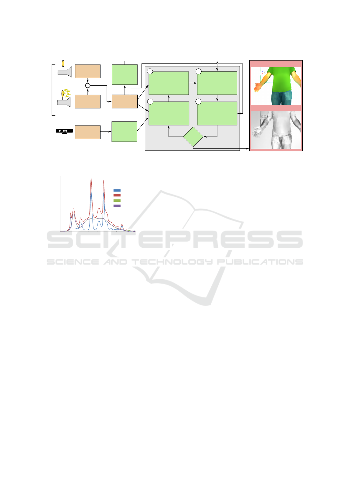
Figure 2: Our framework picture. Green boxes represent the different processings of our algorithm. Orange boxes represent

the values given by the sensors at different times. Red box is the result of our algorithm.

380 430 480 530 580 630 680 730 780

Wavelength

Relative radiant power

100

Unknown Ambient

Unknown Ambient + Flash

Flash

Numerical Difference

Figure 3: Blue: Spectrum of a white Lambertian point un-

der the unknown ambient illumination. Red: Spectrum of a

white Lambertian point under unknown ambient illumina-

tion and ﬂash illumination (total spectrum). Green: Spec-

trum of a white Lambertian point under pure ﬂash illumi-

nation. Purple: difference between the total spectrum and

the ambient spectrum, this difference spectrum completely

matches the pure ﬂash spectrum.

Pure Flash Image from Image Pairs. Our goal is

to create a pure ﬂash image from a pair of two images:

a ﬂashed and non-ﬂashed one (also called ambient im-

age). As we record our images with a time sequential

illumination we use the same aperture and exposure

time for the two images. The ﬂashed image can be

recovered by subtracting the ambient image from the

ﬂashed one, provided that the images are linear and

do not contain any underexposed and saturated pix-

els. As shown in Figure 3, to validate this substraction

(to compute the pure ﬂash image) we have captured

a white Lambertian point under several illuminations

with a spectrometer and subtracted the spectrum of

the ambient illumination from the total spectrum (ob-

tained after trigging the ﬂash). This results in a spec-

trum that matches the spectrum obtained with a pure

ﬂash illumination. To make sure that the combination

of the two images of a pair provides a pure ﬂash im-

age, three caveats should be considered: (1) the two

images must be taken with the same camera param-

eters (exposure time, aperture, focal length), (2) the

images have to be linear, (3) the pixels color should

not be saturated nor underexposed in the two images.

Moreover, as a luminous power decreases with the in-

verse squared distance, objects too far away might not

receive enough light energy from the ﬂash illumina-

tion. This restraints the scenario setup to scenes not

too far from the camera.

4 OUR APPROACH

Our approach is summarized in Figure 2. First, our

hybrid setup (a camera, a Kinect and a Flash) is com-

pletely calibrated to register the Kinect depth image

to the RGB camera. The illumination of the scene

is known (pure ﬂash image) thanks to our time se-

quential illumination. Moreover, as we also know the

extrinsic and intrinsics parameters of our setup, we

can project the depth map (provided by the Kinect)

onto a 3D point map in the camera coordinate sys-

tem. Before reﬁning the normal and the reﬂectance

maps, we compute a rough normal map from the raw

depth map provided by the Kinect (Section 4.2). Then

we use the pure ﬂash image to cluster (K-means clus-

tering) the 3D points seen through the pixels camera,

each cluster containing points of nearly the same dif-

fuse reﬂectance (Section 4.1). Then we start our iter-

ative reﬁnement process consisting of 4 steps. In the

ﬁrst step (Section 4.3), we ﬁlter the normal map, the

weights being depended on luminance to preserve ge-

ometry details and coherence. The second step (Sec-

tion 4.4) performs an estimation of a reﬂectance map

from the pure ﬂashed image and the ﬁltered normal

map. In third step (Section 4.4), a ﬁlter is applied to

the reﬂectance map with weights depending on chro-

Shape and Reﬂectance from RGB-D Images using Time Sequential Illumination

537

maticity. During the last step (Section 4.5), the nor-

mal map is reﬁned thanks to a shading least square

minimization that allows to ﬁt our model to the pure

ﬂash image. Finally, we repeat those steps until con-

vergence, say when both the normal and reﬂectance

maps do not vary anymore. Now, we will detail the

differents steps in the following subsections. For con-

venience purpose, as the images and the depths are

registered, from now on, a point is either a pixel p of

an image captured by the camera or the 3D point P

seen through p.

4.1 Chromaticity Assumption

As in (DiCarlo et al., 2001), we suppose that the chro-

maticity of the scene is sparse. This assumption al-

lows us to perform a color segmentation of the scene

based on quadratic chromaticity distance. The seg-

mentation consists in applying a K-means clustering

to the input image so that each pixel is assigned a clus-

ter of a given chromaticity (Figure 4). Each pixel is

projected onto a 3D point with a diffuse reﬂectance.

Each cluster is supposed to contain pixels of nearly

the same diffuse reﬂectance. We initialize the K-

means centers (10 in our current implementation) by

spreading them in the chromaticity gamut. More ro-

bust clustering techniques are left for future work.

Chromaticity Clusters false color

Figure 4: The chromaticity image is used to cluster surfaces

with similar diffuse reﬂectances. We can observe that the

t-shirt, the background and the skin are classiﬁed into dif-

ferent clusters.

4.2 Computing Normal Map from

Quantiﬁed Depth Data

Let us use the raw depth map (captured by the Kinect)

to compute N(p), the normal associated with a pixel

p. To compute this normal, we need to express the

depth changes (δ

(u,v), δ

(u,v)) as follows:

(u,v) = D(u + 1,v) − D (u − 1,v) (5)

(u,v) = D(u,v + 1) − D (u,v − 1) (6)

The normal, associated with the pixel p, can be

estimated as:

(p) =



2 ·

D(p)

0 −δ

(p)



(7)

(p) =



0 2 ·

D(p)

−δ

(p)



(8)

N(p) = T

(p) × T

(p) (9)

where T

(p) and T

(p) are respectively the tangents to

the surface according to the X and Y axes respectively.

Note that, as the Kinect depth map is quantized, it

represents a piece-wise constant approximation of the

real depth map (see Figure 1). Due to this quanti-

zation artifact, most of the normals, computed from

this depth map, will be oriented toward the camera,

which is a poor initial guess for our normal map re-

ﬁnement algorithm. This quantization artifact makes

the normal map noisy. Consequently, to overcome

the quantization artifact and other possible artifacts,

an important part of our algorithm consists in ﬁltering

the normal map. This ﬁltering is detailed in the next

subsection.

4.3 Normal Map Filtering

To remove noise in the normal map, we apply a bilat-

eral ﬁlter to the normals N (computed from the depth

map) to get ﬁltered normals N

(p) =

(p)

∑

s∈Ω(p)

(s, p)N(s) (10)

where W

(p) is a normalization factor, Ω(p) a neigh-

borhood of the pixel p and Ψ

the weighting function.

The expression of the weighting function depends on

the luminance L of the pixels of the pure ﬂash image

and on the normals:

(s, p) = exp

−

(L(p)

−

L(s))

2σ

−

N(p)

−

N(s)

2σ

where σ

and σ

are weighting parameters related to

luminance and normal respectively. Numerical values

used in our experiments are given in the results sec-

tion. The reason of adding the luminance information

in the weighting function is to preserve geometry de-

tails, as the luminance value changes locally with the

normal orientation.

4.4 Reﬂectance Estimation and

Filtering

Let us consider the case of Lambertian surfaces. The

RGB pixel values of p captured by the camera can be

estimated as follows:

I(p) =

(ω

)

· k

(p) · |N(p).ω

| (11)

VISAPP 2016 - International Conference on Computer Vision Theory and Applications

538

, d, ω

are known as the source illumination is con-

trolled, k

(p) is the diffuse reﬂectance of a Lam-

bertian surface. k

is commonly expressed for each

{r,g,b} component. Reﬁning the normal map re-

quires an estimation of those diffuse reﬂectances.

Once the ﬁrst rough estimation of the normals has

been performed, Equation 2 is used to estimate the

reﬂectance map:

(p) =

(ω

)

I(p)

|N(p).ω

, (12)

where I(p) is the {r, g,b} value of a pixel of the

pure ﬂash image and I

the intensity of the ﬂash light

source. The reﬂectance map is rough as it is computed

from a rough depth map. However, the pure ﬂash im-

age can help improve the reﬂectance map, provided

that the two following assumptions are satisﬁed:

1. if two points have the same normal, the difference

between their pixel values is only due to albedo

change,

2. the distribution of reﬂectance over the image is

sparse to ensure a reliable segmentation (Sec-

tion 4.1).

According to the two above assumptions, any

albedo change is due to chromaticity change (DiCarlo

et al., 2001), in other words any chromaticity change

entails an albedo change. Consequently, the impact of

normal aberration, on the reﬂectance map, can be re-

duced by averaging the diffuse reﬂectances of points

lying in a neighborhood. This averaging operation is

performed using another bilateral ﬁlter:

(p) =

(p)

∑

s∈Ω(p)

(s, p)k

(s) (13)

where W

(p) is the normalization factor, Ψ

being the

weighting function which depends on chromaticity

similarities. Indeed, if two points are not assigned the

same chromaticity cluster (Section 4.1), their weights

are set to zero. The condition that two pixels p and s

belong to the same cluster is:

C(s, p) = (C(s) = C(p)) and (|m(s) − m(p)| < t

)

where C(p) is the cluster id associated with pixel p,

m(p) is the maximum of the r,g,b values of the pixel

p and t

a threshold value that we set to 0.5. The

second term is added to make the distinction between

black and white points. Finally, the expression of the

weight used in Equation 13 is given by:

(s, p) =

(

exp



−

m(s)−m(p)

2σ



if C(s, p)

0 otherwise

where σ

is a weighting parameter. Numerical val-

ues used in our experiments are given in the results

section. To avoid that black, white and grey pixels

mingle during the ﬁltering process, we use a weight

which depends on the maximum m of the r,g,b val-

ues of each pixel.

4.5 Normal Map Reﬁnement

Once the reﬂectance map ﬁltered, the next step con-

sists in reﬁning the normal map. Our reﬁnement relies

on the lambertian model and a least-square error like

algorithm for the three channels of each pixel. Equa-

tion 4 can be written as:

I(p) =

(ω

) · k

(p)

· (N

+ N

) (14)

Let us assume that the right k

reﬂectances are avail-

able, the goal is to ﬁnd the three components of nor-

mal N that minimize ξ over the set of the three rgb

components:

ξ(p) =



∑

(S (p,c) − (N

+ N

))



S (p,c) =

I(p,c) · d

(p, c) · I

(ω

)

where k

(p, c) and I(p,c) are respectively the diffuse

reﬂectance and the value of pixel p for the color chan-

nel c. We want to ﬁnd the minimum error with respect

to (N

), which is reached when:

∂ξ

∂N

(p) = 0 → N

∑

(S (p,c) − N

− N

)

3 · ω

∂ξ

∂N

(p) = 0 → N

∑

(S (p,c) − N

− N

)

3 · ω

∂ξ

∂N

(p) = 0 → N

∑

(S (p,c) − N

− N

)

3 · ω

In the minimization process, each normal N =





is initialized with the rough normal

map computed from he Kinect depth data, then each

component of the normals is computed through an it-

erative scheme until convergence.

4.6 Global Convergence

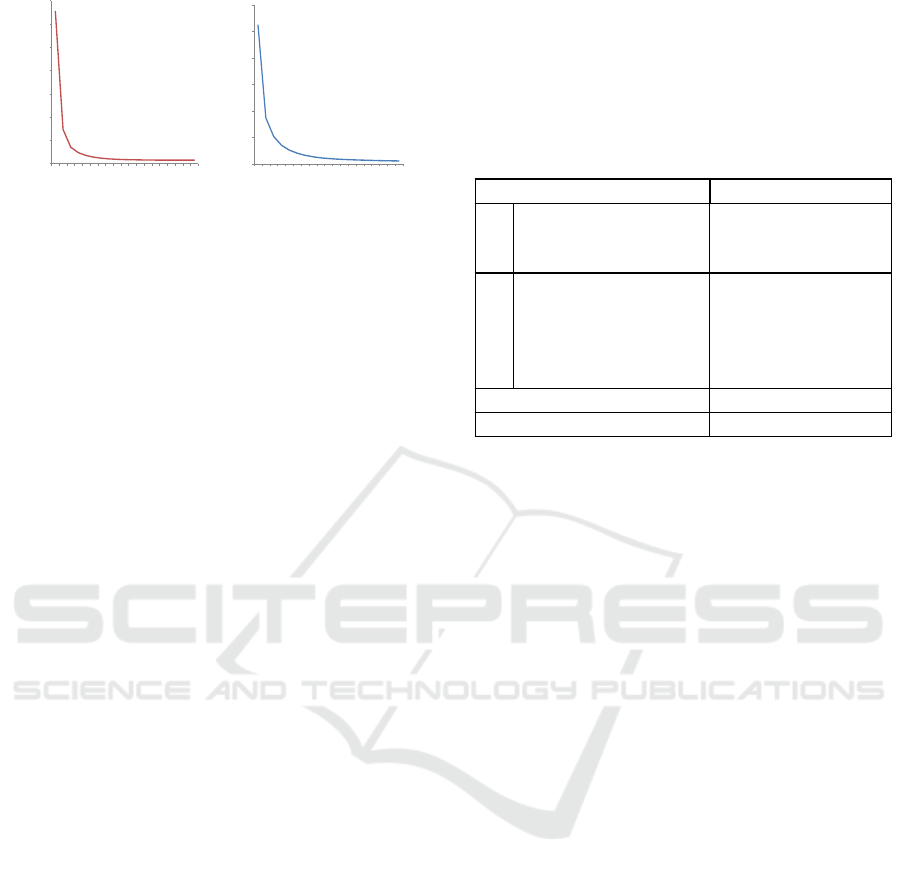
The plots on Figure 5 illustrate the convergence of

the Normal Map and the diffuse reﬂectance map when

applying our iterative algorithm. We computed the

mean distance between the normal map (respectively

the diffuse reﬂectance map) evaluated at the current

iteration and the normal map (respectively the diffuse

reﬂectance map) evaluated at the preceding iteration.

Shape and Reﬂectance from RGB-D Images using Time Sequential Illumination

539

Diffuse Coefﬁcients

Normals

0.12

0.10

0.08

0.06

0.04

0.02

Mean distance

Number of Iterations

Figure 5: Plots representing the convergence of Normals

and Diffuse Reﬂectances for each iteration.

Figure 5 demonstrates that only a few iterations

are necessary to reach a steady state. Indeed, only

4 − 5 iterations are necessary to reach a high quality

Normal and reﬂectance maps.

5 RESULTS

Our experimental setup consists of: a Kinect depth

sensor (depth res. 640 × 480, frame rate 30 fps), a

Ueye Industrial Camera (res. 1280 × 960, frame rate

60 fps with a global shutter) and a ﬂash LED light.

An electronic board is used to synchronize the camera

with the ﬂash. This allows to sequentially acquire an

image pair: ﬂashed and non ﬂashed. So, we are able

to generate an image pair at 30 fps. The Kinect is not

synchronized due to its own limitations. The depth

image is upsampled to match the camera resolution.

We have implemented our technique in C++ and

used CUDA 6.5 to speedup all the steps of our al-

gorithm. The details of the algorithm timings are

summarized in Table 1. All the timings in this ta-

ble have been measured on an a Xeon ES 2640 CPU

2.50GHz×2 (32GB Ram) and an Nvidia Geforce

GTX 580. Note that the image registration step is

not included into our timings. Indeed, its perfor-

mance depends on the setup and the chosen technique.

For example, in (Or-El et al., 2015), this operation

takes 31.1 ms per frame on an Nvidia Titan GPU.

The algorithm parameters were set to: σ

= 0.002,

= 0.0004 and σ

= 0.02 , these values were car-

ried throughout all experiments. For the two ﬁltering

operations (normal and reﬂectance maps), we use a

kernel of 20 pixels size except for the Burger scene

(Figure 6) for which we use a kernel of 10 pixels size.

This is due to the fact that the image of this scene is

twice smaller than that of the other test scenes (Fig-

ure 1 and 8).

Our method is compared to (Or-El et al., 2015).

To this end, we used the Matlab code provided by

the authors. Their method aims at enhancing a depth

map by fusing intensity and depth information to cre-

Table 1: Timings of each step of our algorithm. Bold tim-

ings are obtained using the performance improvement de-

scribed in the next subsection. To compute the total time,

we need to multiply the reﬁnement iteration time by the

number of iterations needed to converge to the desired re-

sults. In practice, only 5 iterations are required, which cor-

responds to 5.84 fps or 0.23 fps on a GTX 580 using or not

using the performance improvement. Note that the ”Image

Alignment” step timing is taken from (Or-El et al., 2015).

Operations Time (ms)

Init.

Image Alignment

∗

31.1

Chroma Clustering 7.34

3D Points Estim. 0.24

Reﬁne iter.

Normal Filtering 495.55 (0.43)

Dot Calculation 0.70

Reﬂectance Estim. 0.26

Reﬂectance Filtering 345.74 (17.39)

Normal Reﬁnement 7.72

Total Reﬁnement Iteration 849.97 (26.5)

Total Time (5 iterations) 4288.53 (171.18)

ate detailed range proﬁles. For this purpose, they

use a lighting model that can handle natural illumi-

nation. This model is integrated in a shape-from-

shading technique to improve the reconstruction of

objects. Note that, unlike our method, their approach

reﬁnes the depths rather than the normals.

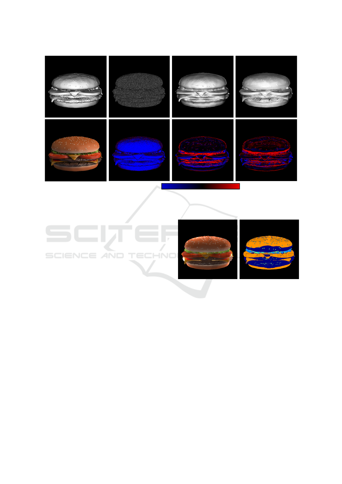
Figure 6 shows a comparison between our method

and the one of (Or-El et al., 2015) for a synthetic

Burger scene. The input depth map is perturbed

by adding a gaussian white noise. To use our al-

gorithm, we rendered the scene using a small light

source that simulates the ﬂash. Our method produces

results with an error smaller than the one obtained

with the method of (Or-El et al., 2015). This is par-

ticularly visible on the tomatoes where ﬁne details are

well recovered. However, there is more noise on the

bread due to clustering issues (Figure 7).

The scene (Figure 8), is a real scene with rela-

tively slow arm movements. Unlike the method of

(Or-El et al., 2015) no mask is used to select the main

object. The input depth map is noisy as it is directly

provided by the Kinect sensor. This noise is different

from the synthetic one used in Figure 6. Compared

to (Or-El et al., 2015), our method provides results

that have less artifacts and ﬁne geometry details are

correctly recovered. The main issue of (Or-El et al.,

2015) method is the use of a bilateral ﬁlter which

is applied to ﬁlter a lot of data due to the high level

of noise in the raw depth map. Our two ﬁltering

operations are performed using bilateral ﬁlters. But,

as we use them at each iteration, a smaller kernel

size is needed, which reduces the artifacts inherent

in large kernel bilateral ﬁlters. Furthermore, at each

iteration we compute new normals (Normal Reﬁne-

VISAPP 2016 - International Conference on Computer Vision Theory and Applications

540

Reference Noisy depth map Or-El et al. 2015 Our method

RGB image

RMSE: 0.668 RMSE: 0.285 RMSE: 0.275

Negative

Positive

Noisy depth map Or-El et al. 2015 Our method

Figure 6: The original burger scene used in (Or-El et al., 2015). Top row show the dot product image (dot product between

the normal and the view direction) using the normals of: the reference solution, the noisy map used as input, (Or-El et al.,

2015) and our method. Bottom row show the RGB image and the false color error on the normal dot product. For better

visualisation the error was multiplied by 3.

ment operation) and new reﬂectances (Reﬂectance

Estimation operation). Consequently, artifacts due

to successive bilateral ﬁltering operations are avoided.

Performance Improvement. One of the bottle-

neck of our algorithm is the two ﬁltering operations

(Normal Filtering and Reﬂectance Filtering) which

take 495.553 ms and 345.74 ms respectively. These

two operations use non separable ﬁlters, which are

time consuming. However, to reduce the computing

time, those ﬁlters can be approximated by separable

ﬁlters with weights carefully computed. The error

due to those approximations are hardly visible. The

computing times needed by the separable version of

these two ﬁlters are 0.49 ms (1005× faster) and 17.39

ms (20× faster). All the timings are summarized in

Table 1. Except for the Burger scene, due to the

reduced image size, this optimization has been used

for all the scenes (Figures 1 and 8). Better and more

robust optimization is left for future work.

Application. One direct application of our algo-

rithm is the relighting of a captured scene. Indeed,

our algorithm provides the reﬂectance and the normal

maps of a scene that we relight with artiﬁcial light

sources (Figure 9). In this scene, the movement of the

arms is fast. This explains the artifacts on the arms

due to motion blur.

Clusters false color

Reflectance refined

Figure 7: On the left: the reﬁned reﬂectance map after con-

vergence of our algorithm. On the right: false color image

to show how the chromaticity-based clustering performs.

We can observe that the tomatoes and the bread lie in the

same cluster. However, due to the local nature of the ﬁlter-

ing, these two material have not been merged.

6 CONCLUSIONS

We showed that even with a consumer camera and a

Kinect (capturing noisy depth data) it is possible to re-

cover ﬁner geometry and precise diffuse reﬂectances

from an image or a video thanks to the use of se-

quential illumination provided by a ﬂash. A pair of

two images are captured: one non ﬂashed image (im-

age under ambient illumination) and a ﬂashed one. A

pure ﬂash image is computed by substracting the non

ﬂashed image from the ﬂashed image. We proposed

an efﬁcient iterative algorithm to recover shapes and

Shape and Reﬂectance from RGB-D Images using Time Sequential Illumination

541

Raw data Or-El et al. 2015 Our method

Our method

Figure 8: T-Shirt scene captured by our setup. From left to right: The raw data display using the dot product, (Or-El et al.,

2015) using the dot product, our method with the dot product and the reﬂectance map.

Pure flash image Religthing 1 Relighting 2

Figure 9: The normal and reﬂectance maps reﬁned by our

algorithm can be used for relighting a scene. Images Re-

lighting 1 & 2 are obtained with different artiﬁcial light

source positions. Moreover, sequential lighting makes our

technique capable of capturing video sequences. However,

fast and large movements in the video could create artifacts

due to motion blur.

reﬂectances from the pure ﬂash image. The fact of

knowing the illumination (ﬂash light source) makes

the extraction of normals and reﬂectances easier and

more efﬁcient. Indeed, as the position and the pho-

tometry of the ﬂash light source is known, we used a

local illumination model to express the normal and the

diffuse reﬂectance for each pixel. From the computed

normals we used the illumination equations to deter-

mine the reﬂectances. In turn, these reﬂectances are

fed to a process that determines new normals. This

process is repeated until convergence. We showed

that only a few iterations are needed to converge to

the desired results.

REFERENCES

Bruckstein, A. M. (1988). On shape from shading.

Computer Vision, Graphics, and Image Processing,

44(2):139–154.

de Decker, B., Kautz, J., Mertens, T., and Bekaert, P. (2009).

Capturing multiple illumination conditions using time

and color multiplexing. In 2009 IEEE Computer

Society Conference on Computer Vision and Pattern

Recognition (CVPR 2009), 20-25 June 2009, Miami,

Florida, USA, pages 2536–2543.

Debevec, P. (2012). The light stages and their applications

to photoreal digital actors. SIGGRAPH Asia Technical

Briefs.

DiCarlo, J. M., Xiao, F., and Wandell, B. A. (2001). Illu-

minating illumination. In Color and Imaging Confer-

ence, volume 2001, pages 27–34. Society for Imaging

Science and Technology.

Diebel, J. and Thrun, S. (2005). An application of markov

random ﬁelds to range sensing. In Advances in neural

information processing systems, pages 291–298.

Fanello, S. R., Keskin, C., Izadi, S., Kohli, P., Kim, D.,

Sweeney, D., Criminisi, A., Shotton, J., Kang, S. B.,

and Paek, T. (2014). Learning to be a depth camera

for close-range human capture and interaction. ACM

Transactions on Graphics (TOG), 33(4):86.

Hern

andez, C., Vogiatzis, G., Brostow, G. J., Stenger, B.,

and Cipolla, R. (2007). Non-rigid photometric stereo

with colored lights. In ICCV.

Higo, T., Matsushita, Y., and Ikeuchi, K. (2010). Consen-

sus photometric stereo. In Computer Vision and Pat-

tern Recognition (CVPR), 2010 IEEE Conference on,

pages 1157–1164. IEEE.

Horn, B. K. (1970). Shape from shading: A method for

obtaining the shape of a smooth opaque object from

one view.

Horn, B. K. and Brooks, M. J. (1989). Shape from shading.

MIT press.

Kim, H., Wilburn, B., and Ben-Ezra, M. (2010). Photomet-

ric stereo for dynamic surface orientations. In Com-

puter Vision - ECCV 2010, 11th European Confer-

ence on Computer Vision, Heraklion, Crete, Greece,

September 5-11, 2010, Proceedings, Part I, pages 59–

72.

Nehab, D., Rusinkiewicz, S., Davis, J., and Ramamoorthi,

R. (2005). Efﬁciently combining positions and nor-

mals for precise 3d geometry. ACM transactions on

graphics (TOG), 24(3):536–543.

Newcombe, R. A., Fox, D., and Seitz, S. M. (2015). Dy-

namicfusion: Reconstruction and tracking of non-

rigid scenes in real-time. In Proceedings of the IEEE

Conference on Computer Vision and Pattern Recogni-

tion, pages 343–352.

Or-El, R., Rosman, G., Wetzler, A., Kimmel, R., and Bruck-

stein, A. M. (2015). Rgbd-fusion: Real-time high pre-

cision depth recovery. In Proceedings of the IEEE

Conference on Computer Vision and Pattern Recog-

nition, pages 5407–5416.

Petschnigg, G., Szeliski, R., Agrawala, M., Cohen, M.,

Hoppe, H., and Toyama, K. (2004). Digital photogra-

phy with ﬂash and no-ﬂash image pairs. ACM trans-

actions on graphics (TOG), 23(3):664–672.

Prados, E. and Faugeras, O. (2005). Shape from shading: a

well-posed problem? In Computer Vision and Pattern

VISAPP 2016 - International Conference on Computer Vision Theory and Applications

542

Recognition, 2005. CVPR 2005. IEEE Computer So-

ciety Conference on, volume 2, pages 870–877. IEEE.

Richardt, C., Stoll, C., Dodgson, N. A., Seidel, H.-P., and

Theobalt, C. (2012). Coherent spatiotemporal ﬁlter-

ing, upsampling and rendering of rgbz videos. In

Computer Graphics Forum, volume 31, pages 247–

256. Wiley Online Library.

Shen, L., Tan, P., and Lin, S. (2008). Intrinsic image de-

composition with non-local texture cues. In Computer

Vision and Pattern Recognition, 2008. CVPR 2008.

IEEE Conference on, pages 1–7. IEEE.

Shen, L. and Yeo, C. (2011). Intrinsic images decomposi-

tion using a local and global sparse representation of

reﬂectance. In Computer Vision and Pattern Recogni-

tion (CVPR), 2011 IEEE Conference on, pages 697–

704. IEEE.

Tunwattanapong, B., Fyffe, G., Graham, P., Busch, J., Yu,

X., Ghosh, A., and Debevec, P. (2013). Acquiring

reﬂectance and shape from continuous spherical har-

monic illumination. ACM Transactions on graphics

(TOG), 32(4):109.

Wenger, A., Gardner, A., Tchou, C., Unger, J., Hawkins,

T., and Debevec, P. (2005). Performance relighting

and reﬂectance transformation with time-multiplexed

illumination. 24(3):756–764.

Woodham, R. J. (1980). Photometric method for determin-

ing surface orientation from multiple images. Optical

Engineering, 19(1):191139–191139–.

Wu, C., Zollh

ofer, M., Nießner, M., Stamminger, M., Izadi,

S., and Theobalt, C. (2014). Real-time shading-based

reﬁnement for consumer depth cameras. Proc. SIG-

GRAPH Asia.

Xiao, F., DiCarlo, J. M., Catrysse, P. B., and Wandell,

B. A. (2001). Image analysis using modulated light

sources. In Photonics West 2001-Electronic Imag-

ing, pages 22–30. International Society for Optics and

Photonics.

Shape and Reﬂectance from RGB-D Images using Time Sequential Illumination

543