A Prototype Application for Long-time Behavior Modeling and
Abnormal Events Detection
Nicoletta Noceti and Francesca Odone
DIBRIS, Universit
`
a degli Studi di Genova, via Dodecaneso 35, Genova, Italy
Keywords:
Behaviour Modelling, Abnormal Events Detection, Temporal Series Clustering.
Abstract:
In this work we present a prototype application for modelling common behaviours from long-time observa-
tions of a scene. The core of the system is based on the method proposed in (Noceti and Odone, 2012), an
adaptive technique for profiling patterns of activities on temporal data – coupling a string-based representation
and an unsupervised learning strategy – and detecting anomalies — i.e., dynamic events diverging with re-
spect to the usual dynamics. We propose an engineered framework where the method is adopted to perform an
online analysis over very long time intervals (weeks of activity). The behaviour models are updated to accom-
modate new patterns and cope with the physiological scene variations. We provide a thorough experimental
assessment, to show the robustness of the application in capturing the evolution of the scene dynamics.
1 INTRODUCTION
The essence of video-surveillance is to be able to
analyse a scene for very long time frames and to au-
tomatically detect anomalous events. In contrast, re-
searchers often refer to short benchmark video se-
quences when analysing the performances of their
methods. For this reason it is rather difficult to es-
timate the robustness of a method with respect to the
natural evolution of a scene along time. In spite of
the considerable amount of work carried out until now
(Johnson and Hogg, 1995; Bulpitt and Sumpter, 2000;
Javed and Shah, 2004; Hu et al., 2007), real video-
surveillance systems are still relying heavily on inputs
from human operators. In practice, when a new sys-
tem is installed, a configuration which highlights for-
bidden behaviours is mandatory. We are still missing
automatic procedures able to assist the user in defin-
ing patterns of common behaviours, suggesting situa-
tions of potential danger.
This paper presents an engineered prototype of a
monitoring application, the core of which is based on
the theoretical model proposed in (Noceti and Odone,
2012). Such a model, which may be applied to dif-
ferent video analysis tasks, relies on the availabil-
ity of a set of trajectories to describe meaninfull dy-
namic events occurring in a scene. Then, unsuper-
vised learning is adopted to build models of com-
mon patterns of activities in the environment by ex-
ploiting a string-based representation and a clustering
approach from long-time observations of the scene
dynamics. As a side effect, the model provides the
means to detect anomalous events.
Here we apply the model to a video-surveillance
setting. Our goal is to produce an adaptive model of
behaviours that are common in the observed scene.
Dynamic events observed over a long temporal span
are used to first initialise a model of common be-
haviours and then update it over time if it is needed.
We discuss different strategies to update the be-
haviour models over time, to accomodate the effects
of scene variations. Unlike in our previous works, the
experimental procedure we adopt here is online and it
incorporates new behaviour models when necessary.
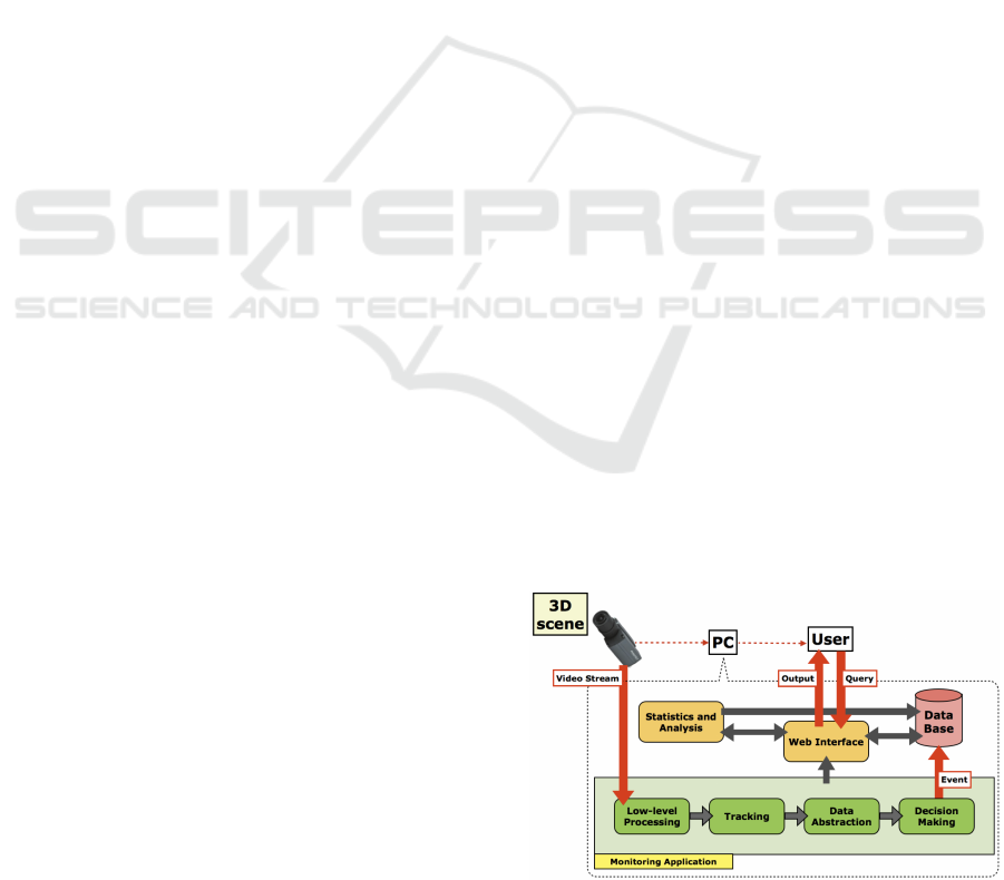
Figure 1 shows a visual representation of the pro-
totype monitoring system. The video-surveillance
Figure 1: A visual representation of the prototype monitor-
ing application.
Noceti, N. and Odone, F.
A Prototype Application for Long-time Behavior Modeling and Abnormal Events Detection.
DOI: 10.5220/0005723105970604
In Proceedings of the 11th Joint Conference on Computer Vision, Imaging and Computer Graphics Theory and Applications (VISIGRAPP 2016) - Volume 4: VISAPP, pages 597-604
ISBN: 978-989-758-175-5
Copyright
c
2016 by SCITEPRESS – Science and Technology Publications, Lda. All rights reserved
597

camera
1
is connected to a computer in which a de-
voted software organises the acquisitions and runs the
monitoring application. The analysis in performed
continuously over time.
When a new dynamic event is observed and clas-
sified, an event is generated and described with a set
of tags – including type of event (normal event with
information on the assigned class, or anomaly), start-
ing and ending time, description, ... – which are col-
lected on a data base. The final user can constantly
monitor the system status via a web machine-user in-
terface, where the intermediate output of each stage of
the pipeline can be visualised. Moreover, the user is
allowed to formulate queries to the data base to anal-
yse the results and obtain statistics.
Previous Works. Profiling behaviours from tempo-
ral data is a research domain with a long history,
where the benefit of adopting machine learning tech-
niques has soon been observed. The problem has
been tackled using supervised methods, as Support
Vector Machines (Chen and Aggarwal, 2011) or Hid-
den Markov Models (F. Bashir and Schonfeld., 2007).
However many applications– in particular within the
video analysis domain– are characterised by the avail-
ability of huge sets of data but relatively few labeled
ones; therefore an increasing interest has been posed
to the unsupervised perspective. A rather complete
account of event classification in an unsupervised set-
ting is reported in (Morris and Trivedi, 2008); see also
(Stauffer and Grimson, 2000; Hu et al., 2006).
More recently, there has been a renewed attention
on the problem of detecting abnormal events. We cite
for instance the work in (Cheng et al., 2015), where
a local and global anomalies are detected using a re-
gression model on Spatio-Temporal Interesting Points
(STIPs), (Ren et al., 2015) that employs Dictionary
Learning to build models of common activities, or
again (Xu et al., 2015), which is built on top of the
by now popular Deep Neural Networks.
2 MONITORING APPLICATION
We address the problem of modelling behaviours in a
setting where people are observed as a whole and their
dynamic can be described by a trajectory of temporal
observations. A behaviour can then be formalised as a
set of dynamic events coherent with respect to a cer-
tain metric (e.g. going from a point A to point B or
1
The video surveillance setup has been obtained
within a technology transfer program with Imavis S.r.l.,
http://www.imavis.com.
enter the region C). Depending on the available infor-
mation on the trajectories, more subtle properties can
be enhanced, e.g. if velocity is considered, then the
behaviour going from A to B can be further divided
into going from A to B by walking or by running.
In the following we describe our monitoring applica-
tion. On a first period, we simply collect dynamic
events representations, and then run the training stage
in batch to obtain an initial guess on the patterns of
common activity in the scene. The core of this step is
the method we proposed in (Noceti and Odone, 2012),
summarised in Sec. 2.1 and 2.2 (we refer to the orig-
inal paper for further details). Then, the online test
analysis starts. If necessary, the behaviours models
are updated to address the problem of adapting to the
scene changes. We discuss this point if Sec. 2.3.
2.1 Modelling Common Activities in a
Scene
The method we adopt consists of different steps. A
low-level processing collects trajectories over time,
which in a second step are mapped into strings rep-
resentations. Finally, groups of coherent strings are
detected with clustering.
2.1.1 Low-level Video Processing
Our low-level processing (Noceti et al., 2009) aims
first at performing a motion-based image segmenta-
tion to detect moving regions (see Fig. 2(b)), that
in our setting can be associated with a single per-
son or a small group of people (see Fig. 2(c)). At
a given time instant t, each moving object i in the
scene is described according to a vector of feature
x
t
i
= [P
t
i
,S
t
i
,M
t
i
,D
t
i
] ∈ R
5
, where P denotes the object
position in the image plane, S its size, M and D the
magnitude and orientation of the object motion.
The tracking procedure correlates such vectors
over time (Fig. 2(c)), obtaining N spatio-temporal tra-
jectories that are collected on a training set of tempo-
ral series X = {x
i
}
N
i=1
.
2.1.2 String-based Trajectory Representation
We map each temporal trajectory into a new repre-
sentation based on strings – formally, a concatena-
tion of symbols from a finite alphabet A . The al-
phabet can be obtained by partitioning the space of
all vectors x
t
i
disregarding the temporal correlation:
˜
X = {{x
t
i
}
k
i
t=1
}
N
i=1
, where k
i
refers to the length of the
i-th trajectory. We adopted the method proposed in
(Noceti et al., 2011), where the benefit of adopting a
strategy guided by the available data, as opposed to
VISAPP 2016 - International Conference on Computer Vision Theory and Applications
598

(a) (b) (c)
Figure 2: The low-level processing of the monitoring system, based on (Noceti et al., 2009): each frame (left) is first segmented
to detect moving regions (center). Then each region is described with a feature vector used in the tracking process to assign
and maintain the identity of the subject or group of people (right).
a manual or a regular grid has been discussed. The
partition method relies on clustering data in
˜
X with a
recursive implementation of spectral clustering (Shi
and Malik, 2000). A nice property is that it does not
require to fix a priori the number clusters, while still
allows to influence the granularity of the solution with
appropriate parameter tuning.
As for the similarity measure, we adopt the func-
tion proposed in (Noceti et al., 2011), based on a con-
vex combination of kernel-based similarity functions
computed on sub-sets of coherent features:
G(x
1
,x
2
,w,θ) =w
P
G
P
(P
1
,P
2
,σ
P
)+
w
S
G
S
(S
1
,S
2
,σ
S
)+
w
M
G
M
(M
1
,M
2
,σ
M
)+
w
D
G
D
(D
1
,D
2
,σ
D
),
(1)
where w = {w
P
,w
S
,w
M
,w
D
} are the feature weights,
while {G
P
,G
S
,G
M
,G
D
} are Gaussians with standard
deviations θ = {σ
P
,σ
S
,σ
M
,σ
D
} and zero means.
Once that the clustering has been performed, a set
of states composing the features partition is available.
The alphabet can be finally obtained by associating a
symbol with each state.
At this point, a temporal series x
i
can be translated
into a string s. Each element x
t
i
∈ R
5
is compared
(using again Eq. 1) with the centroid of the states.
Then, the element is represented in the string by the
label associated with the closest state. We now have
obtained the set S = {s
i
}
N
i=1
, composed by the string
representations of the original training set X.
2.1.3 Behavior Modeling using Strings
Clustering
The method we adopt to discover patterns of common
activities includes three steps: (i) strings clustering,
(ii) candidates selection, and (iii) clusters refinement.
Step (i) is again based on Spectral Clustering,
which is run on the strings representation with the
aim of detecting groups of coherent strings. To eval-
uate the similarity between strings we adopt the P-
spectrum kernel (see (Taylor and Cristianini, 2004)).
The peculiarities of our data reside on the transitions
between states, thus we set P = 2 and discard the
replicated symbols from each strings before applying
spectral clustering. We refer the interested reader to
(Noceti and Odone, 2012) for the theoretical justifica-
tions.
We now have a string partition B, defining groups
of coherent temporal events, including the strings
clusters {S
1
,...,S
|B|
}. To represent each of them in
a compact way we select a cluster candidate with a
voting strategy (step (ii)). In what follows, we will
refer to the candidate of strings cluster S
i
with ˆs
i
. In-
tuitively, the candidate string can be interpreted as an
“average” string within a cluster. Only the votes cor-
responding to a high similarity are considered: notice
that this is equivalent to discard outliers from clus-
ters before candidates selection, obtaining a method
which is tolerant to the presence of noisy data.
Given the strings partition B, a refinement stage
(step (iii)) is applied to improve the quality of clus-
ters, given that Spectral Clustering may produce over-
segmented results on real, noisy data. To this pur-
pose, first low-quality clusters (groups with either a
low intra-class similarity or a small cardinality) are
removed. Then, clusters with very similar candidates
are merged.
2.2 Model Selection with Loose Prior
Information
The choice of parameters influences the obtained
models, thus it is worth discussing how to appropri-
ately assign their a value. In our case, they include
the weights w (see Eq. 1) and the parameters used for
Spectral Clustering to control the granularity of the
solution (the so-called cut thresholds, referred to as
τ
A
for the alphabet and τ
S
for the strings partition).
When a ground truth is available, then the best clus-
tering solution may be chosen by solving a 1-to-1 as-
signment problem between estimated clusters and ex-
pected clusters. However, in many real circumstances
A Prototype Application for Long-time Behavior Modeling and Abnormal Events Detection
599

with the availability of huge amounts of data, obtain-
ing a manual and full annotation might be painful and
generate very subjective views of the problem.
We adopt instead a viable strategy which involves
the annotation of the observed environment, rather
than of the dynamic events. To goal is to manually
identify regions of the scene which are characterised
by some level of relevance (as in presence of doors
of coffee urns). Figure 5 shows an example of an an-
notation for the scene used in our experiments. We
refer to this annotation as a loose annotation, in that
it provides a partial annotation of the dynamic events,
which are grouped according to starting point (source
region) and final point (sink region). It goes that only
spatial properties influence the annotation, and as a
consequence it may generate heterogeneous groups:
trajectories sharing source and sink regions may cor-
respond to different classes of objects or motion type
– e.g. the event going directly from the source to
the sink will be grouped together with events cross-
ing other intermediate regions.
For these reasons, a 1-to-N mapping is more ap-
propriate to our case: an annotated cluster is allowed
to be associated with multiple estimated clusters to
avoid high penalties for over-segmented but reason-
able results (Brox and Malik, 2010). In fact, since
the ground truth only relies on spatial properties, an
annotated cluster may be split in more than one esti-
mated clusters because other properties are captured
(e.g. people walking vs people running, people vs
cars, ...). Hence, an estimated cluster is always as-
sociated with the ground truth cluster with highest in-
tersection.
We compute the Correct Clustering Rate (CCR)
(Morris and Trivedi, 2009) to evaluate the goodness
of a given clusters mapping. Consequently, model se-
lection simply implies to select the parameters that
maximize such value.
2.3 Evolving the Models over Time
After the training stage the system starts to monitor
the scenario analysing the new observed events. The
training stage described so far is batch, thus models
are maintained as they have been estimated during
training. Instead, it goes that the models should be
able to automatically update to cope with the tempo-
ral variations in the scene.
The models might be updated at fixed intervals –
e.g. each night or in the week-end to avoid system
overloading during daytime analysis – or when the
performances significantly decrease. In an unsuper-
vised setting there is no direct way to evaluate such
deterioration, but we may consider a constantly in-
creasing amount of detected anomalies as an indica-
tion of the fact models might be becoming obsolete.
In our scenario, if the number of dynamic events as-
sociated with known models is very low then it might
be the case to replicate the entire training pipeline,
since some features may had acquired importance
with respect to others and thus the alphabet to build
the string-based representation may be varied. How-
ever, usually we can assume the alphabet is still valid,
while the patterns of activities may be more affected
by variations in the scene.
Starting from the strings in the original training
set, we refer to as S
0
= {s
i
}
N
0
S
i=0
, from which the parti-
tion C
0
= {C
0
i
}
N
0
C
i=1
of N
0
C
clusters have been estimated
and represented via the set of candidates c
0
= {c
0
i
}
N
0
C
i=1
,
we first discard the strings in S
0
whose similarity with
their candidates is below a threshold. Then we add the
new observed strings S
∆t
= {s
j
}
N
∆t
S
j=0
over a temporal
window of ∆t frames: the interval under considera-
tion should cover the period occurred since the last
update (or the training stage). If the number of strings
considered in this way is too high the clustering steps
becomes computationally unfeasible, and thus a ran-
dom sampling can be applied. Since the new train-
ing stage involves the strings clustering step only, the
model selection procedure is limited to the choice of
the corresponding cut threshold, τ
S
.
3 LEARNING BEHAVIORS:
LONG-TERM EXPERIMENTS
In this section we discuss the performances of our ap-
proach to behaviour modeling over the long time pe-
riod. The monitored environment, shown in Fig. 5,
is one of the main hall of our department. The en-
vironment consists in an indoor open space where a
good amount of dynamic events occur during day-
time. Only people are supposed to be moving in the
scene, in which the complexity depends on several
factors, as level of crowd or illumination changes.
The analysis is performed over a period of 7
weeks, characterised by a different amount of dy-
namic activity. The storyline of the scene is depicted
in Fig. 3. On the first week, where normal activ-
ity can be observed, we simply collect data and train
our initial models. On the second and third weeks,
characterised by a normal activity as well, we test our
model. We expect a few anomalies to be identified in
this period. On the fourth week a special event occurs
(the department was open to high school students),
and some structural variations are applied to the scene
VISAPP 2016 - International Conference on Computer Vision Theory and Applications
600

during the week (tables and bulkheads are temporary
rearranged, camera position slightly changes). As a
consequence we expect that both the amount of ob-
served dynamic events and detected anomalies in-
crease. To follow, there are two weeks of holidays,
in which very few dynamics should be observed, to
go back to a normal activity on the last week of anal-
ysis. In this last week exam sessions took place, with
a consequent significant activity in the area of the ta-
ble (due to students studying).
We now detail the temporal analysis.
3.1 Training the Initial Models
We collected data for training the initial models over
the first week, gathering a training set of 1203 dy-
namic events, loosely annotated according to the 9
source-sink regions reported in Fig. 5.
The model selection procedure selected as best pa-
rameters W
P
= 0.5, W
S
= 0.1, W
M
= 0.2 and W
D
= 0.2,
τ
A
= 0.85 and τ
S
= 0.75 (the values of the sigma’s
were σ
P
= 70.278, σ
S
= 5631.8, σ
M
= 1.278 and
σ
D
= 0.597). The model corresponds to a cluster-
ing including the 10 behaviours reported in Fig. 4
and represented with arrows in Fig. 5. It is easy to
observe that the identified patterns can be associated
with rather common and intuitive activities occurring
in the scene.
Notice how the behaviours pairs 2-5 and 6-8 show
a significant spatial overlap. For the latter, an inspec-
tion of the other features indicates the difference be-
tween them which has been embedded in the clus-
tering solution. Indeed, the distributions of the area
feature of all the observations of trajectories included
in the clusters reveal rather different average values
(∼ 1500 for pattern 6, ∼ 3000 for pattern 8) that may
refer to single subjects and small groups, respectively.
The separation of the pair 2-5 is likely to be due to an
over-segmentation of the data. However, trajectories
included in pattern 2 show a higher spatial compact-
ness, which is also reflected in the distribution of the
direction features (characterised by a very low stan-
dard deviation).
3.2 Run-time Analysis
In this section we discuss the run-time analysis: given
the models estimated after the training stage the sys-
tem acquires new observations, describes the dynamic
events according to the scheme representation fol-
lowed during training and adopting the parameters se-
lected as best performing, and finally tries and asso-
ciate the new datum with one of the known models.
The association follows a Nearest Neighbour strat-
egy: the new datum, represented as string, is com-
pared with all the known models, i.e. their candidates.
If no candidate has a high similarity (above a thresh-
old, 0.6 in our experiments) with the new string, then
the new event is considered anomalous.
Let us first have a look at the number of events
observed during the period of analysis: the plot, re-
ported in Fig. 6(a) shows that the trends of each week
present a rather similar shape, with peaks in the mid-
dle (Wednesday’s). Also, the weeks just before and
after the holidays show a higher amount of activity.
After the first week of training, we performed the
classification analysis over the remaining weeks, with
the aim of discriminating between normal dynamics
and anomalies. The analysis is extensively discussed
on the next sections.
3.2.1 With Fixed Models
As a baseline, we adopted the models estimated dur-
ing training over the whole period of analysis (no up-
dating).
Figure 6(b) reports the number of anomalous
events detected over the weeks, included the statistics
on the first week (training) that serve as a reference
value. The fraction of anomalies detected in the 4th
week is higher than in the previous days, and even
higher after holidays. This is justified by the special
event scheduled during the 4th week, in which the
activities diverged with respect to the common dy-
namics of the environment due to both the presence
of outer people and the variation on the scene struc-
ture. The latter also justifies the presence of many
anomalies after the holidays weeks. Indeed, the av-
erage percentage of anomalies over the weeks (with
the exception of the holidays interval, in which only
a few dynamic events have been observed) shows a
growth over time (W2: 0.12, W3: 0.15, W4: 0.25,
W7: 0.27), suggesting that the initial models may be
becoming more and more obsolete. Notice that al-
though the amount of measured dynamic events is
significantly higher on the last week, the fraction of
anomalous events is comparable to the corresponding
statistics of week 4, where scene variations have been
applied.
This suggests the benefit of updating the initial
models with new observations from the environment.
Possible solutions are discussed in what follows.
3.2.2 With Model Updating
The choice regarding when updating the system can
be done following different criteria, we considered 3
different strategies. The first strategy (Fig. 7(a)) re-
lies on updating the models at fixed time intervals, and
A Prototype Application for Long-time Behavior Modeling and Abnormal Events Detection
601

Figure 3: Storyline of the long-time period of analysis of our prototype application.
(a) B0: A → H (b) B1: G → F (c) B2: H → B (d) B3: H → A (e) B4: I → H
(f) B5: H → B (g) B6: H → F (h) B7: B → H (i) B8: H → F/G (j) B9: E → G
Figure 4: Behaviors learned on the training phase. Source (in green) and sink (in red) locations are also reported.
Figure 5: Patterns of activity detected with the training
stage.
more specifically at the end of each week, during the
week-end, where the computational load of the sys-
tem is significantly lower due to the lack of dynamics
in the scene. The step is performed only when the
amount of observed events is significant. Thus, at the
end of training we have at disposal the initial unsuper-
vised model M0 U, which is updated to model M1 U
at the end of the second week. During holidays no
update takes place due to the scarcity of dynamics.
An alternative to avoid the computational weight
of updating procedures which are not strictly neces-
sary is to update the models when the performances
decrease too much. In our implementation (Fig. 7(b))
we evaluate the percentage of anomalies with respect
to the total number of dynamic events, to trigger a
models update when the amount goes above a given
threshold (here 20%). In the specific experimental
scenario, this corresponds to a unique models update,
performed at the end of week 4.
A third strategy of updating relies on the use of
(a)
(b)
Figure 6: The amount of observed events (above) and of
anomalies detected if no updating rule is applied (below)
during the whole period of analysis.
a different trajectory classifier to be adopted when
the models become stable. Figure 7(c) shows a pos-
sible implementation leveraging on the use of tradi-
tional Support Vector Machine (SVM) equipped with
the P-Spectrum kernel. The training stage considers
the same training set as in the unsupervised counter-
part, with strings labels according to the annotation
induced by the clustering result selected as optimal
(best fitting the loose annotation). A k-fold cross val-
idation (k=5) has been used to select the parameters
VISAPP 2016 - International Conference on Computer Vision Theory and Applications
602

(a)
(b)
(c)
Figure 7: Different strategies for models evolution.
Figure 8: Anomalies detected over time comparing the 3
strategies for models updating.
of SVM’s. In our experimental setting, models are
considered as stable after the second week, so the ini-
tial unsupervised models are employed for training
the supervised model M0 S, which becomes now the
active model adopted for the classification of the new
observed data. At the end of week 4, where a higher
amount of anomalies has been detected, a new train-
ing is performed to estimate the updated unsupervised
models, M1 U, which is converted to the supervised
counterpart only in presence of an appropriate amount
of dynamics and a low rate of anomalies. This corre-
sponds to the end of week 7.
Figure 8 shows the trend of the anomalies percent-
age over the weeks of analysis (with the exception of
holidays) comparing the different update strategies –
we will refer to as NU (no update), S1 (strategy 1),
S2 (strategy 2) and S3 (strategy 3). On the first two
weeks, the performances are equal because the be-
havior models correspond to the original cluster in
all the three strategies. On week 3, the first model
update at the end of week 2 causes a gain in perfor-
mances to S1. The update triggered at the end of the
special event (week 4) is not sufficient to S1 for per-
forming appropriately on the last week. Instead, the
update performed with S2 (at the end of week 4 as
well) guarantees a more stable solution thanks to the
higher amount of dynamic events adopted for the new
training stage (subsampled from the observations of
weeks 2, 3 and 4). This reflects on the fact that the
amount of anomalies detected on week 7 goes back
to the accepted level (below the threshold, in red in
the picture). The supervised classifier employed in
S3 seems to have performances comparable to the un-
supervised counterpart. This suggests that even in the
unsupervised case, where the labels are not explicitly
employed in the modeling stage, the prior information
is appropriately exploited to build models which are
robust to noise.
We conclude with some final remarks on the patterns
detected after the models updating with S2 at the end
of week 4 (Fig. 9(a)) and examples of clusters so in-
cluded in the models while classified as anomalies by
the original learnt patterns (see Fig. 9, below). As ex-
pected, a richer description of the scene dynamics is
achieved.
4 CONCLUSION
In this paper we presented an engineered prototype
of a monitoring application, adopting the method for
behaviour modelling proposed in (Noceti and Odone,
2012). The application is able to collect a low-level
description of a dynamic event in terms of a trajectory,
which is then turned into a string-based representation
that captures the peculiarities of the data. Then, com-
mon patterns of activities are detected adopting un-
supervised learning – and clustering, in particular –
on large sets of dynamic events. During the run-time
analysis, a new dynamic event is described according
to the same procedure, and classified as instance of
one of the known behaviour, or as an event which di-
A Prototype Application for Long-time Behavior Modeling and Abnormal Events Detection
603

(a)
(b) H → I (c) B → C (d) C → H
Figure 9: Above, patterns of activity detected after the mod-
els updating step. Below, examples of obtained clusters.
verges with respect to the normality, thus an anomaly.
We discussed the use of three different strategies
to update the models, starting from an initial configu-
ration, and evaluated the monitoring application on a
period of seven weeks of analysis. The results show
the robustness of the method over time, which pro-
vides a tolerance with respect to variations in the envi-
ronment. The update of the models allows to accom-
modate for new patterns which are initially associated
with the anomaly class but then turned into a common
activity due to the persistence over time.
REFERENCES
Brox, T. and Malik, J. (2010). Object segmentation by long
term analysis of point trajectories. In ECCV, pages
282–295.
Bulpitt, A. and Sumpter, N. (2000). Learning spatio-
temporal patterns for predicting object behaviour.
IMAVIS, 18(9):697–704.
Chen, C. and Aggarwal, J. (2011). Modeling human activi-
ties as speech. In CVPR, pages 3425–3432.
Cheng, K.-W., Chen, Y.-T., and Fang, W.-H. (2015). Video
anomaly detection and localization using hierarchi-
cal feature representation and gaussian process regres-
sion. In CVPR, pages 2909–2917.
F. Bashir, A. K. and Schonfeld., D. (2007). Object
trajectory-based activity classification and recognition
using hidden markov model. IP, 16(7):1912–1919.
Hu, W., Xiao, X., Fu, Z., Xie, D., Tan, T., and Maybank,
S. (2006). A system for learning statistical motion
patterns. PAMI, 28(9):1450–1464.
Hu, W., Xie, D., Fu, Z., Zeng, W., and Maybank, S.
(2007). Semantic-based surveillance video retrieval.
IP, 16(4):1168–1181.
Javed, I. J. O. and Shah, M. (2004). Multi feature path mod-
eling for video-surveillance. In ICPR, pages 716–719.
Johnson, N. and Hogg, D. (1995). Learning the distribution
of object trajectories for event recognition. In BMVC,
volume 2, pages 583–592.
Morris, B. and Trivedi, M. (2008). A survey of vision-based
trajectory learning and analysis for surveillance. Circ.
and Sys. for Video Tech., 18(8):1114–1127.
Morris, B. and Trivedi, M. M. (2009). Learning trajectory
patterns by clustering: Experimental studies and com-
parative evaluation. In CVPR, pages 312–319.
Noceti, N., Destrero, A., Lovato, A., and Odone, F. (2009).
Combined motion and appearance models for robust
object tracking in real-time. In AVSS, pages 412–419.
Noceti, N. and Odone, F. (2012). Learning common be-
haviors from large sets of unlabeled temporal series.
Image and Vision Computing, 30(11):875–895.
Noceti, N., Santoro, M., and Odone, F. (2011). Learn-
ing behavioral patterns of time series for video-
surveillance. In Learning Behavioral Patterns of Time
Series for Video-Surveillance (Springer), pages 275–
304. Springer-London.
Ren, H., Liu, W., Olsen, S., and Moeslund, T. (2015). Unsu-
pervised behaviour-specific dictionary learning in ab-
normal event detection. In BMVC.
Shi, J. and Malik, J. (2000). Normalized cuts and image
segmentation. Trans. on PAMI, 22(8):888–905.
Stauffer, C. and Grimson, E. (2000). Learning patterns of
activity using real-time tracking. PAMI, 22(8):747–
757.
Taylor, J. S. and Cristianini, N. (2004). Kernel Methods for
Pattern Analysis. Cambridge University Press.
Xu, D., Ricci, E., Yan, Y., Song, J., and Sebe, N. (2015).
Learning deep representations of appearance and mo-
tion for anomalous event detection. In BMVC.
VISAPP 2016 - International Conference on Computer Vision Theory and Applications
604
