
Structured Edge Detection for Improved Object Localization using the
Discriminative Generalized Hough Transform
Eric Gabriel
1
, Ferdinand Hahmann
1
, Gordon B
¨
oer
1
, Hauke Schramm
1,2
and Carsten Meyer
1,2
1
Institute of Applied Computer Science, Kiel University of Applied Sciences, Kiel, Germany
2
Department of Computer Science, Faculty of Engineering, Kiel University (CAU), Kiel, Germany
Keywords:
Object Detection, Object Localization, Feature Extraction, Edge Detection, Canny Edge Detection, Structured
Edge Detection, Discriminative Generalized Hough Transform.
Abstract:
Automatic localization of target objects in digital images is an important task in Computer Vision. The Gen-
eralized Hough Transform (GHT) and its variant, the Discriminative Generalized Hough Transform (DGHT),
are model-based object localization algorithms which determine the most likely object position based on accu-
mulated votes in the so-called Hough space. Many automatic localization algorithms - including the GHT and
the DGHT - operate on edge images, using e.g. the Canny or the Sobel Edge Detector. However, if the image
contains many edges not belonging to the object of interest (e.g. from other objects, background clutter, noise
etc.), these edges cause misleading votes which increase the probability of localization errors. In this paper
we investigate the effect of a more sophisticated edge detection algorithm, called Structured Edge Detector,
on the performance of a DGHT-based object localization approach. This method utilizes information on the
shape of the target object to substantially reduce the amount of non-object edges. Combining this technique
with the DGHT leads to a significant localization performance improvement for automatic pedestrian and car
detection.
1 INTRODUCTION
The first step in many automatic Computer Vision
systems is the localization of objects of interest in a
given digital image. In this paper, object localization
refers to estimating the coordinates of a given refer-
ence point (e.g. the center of gravity) of the target ob-
ject in any test image. A bounding box around the tar-
get object can then be predicted as described in Sec-
tion 3.3. Object localization is a prerequisite for many
subsequent automatic image processing algorithms,
e.g. automatic segmentation of organ structures in
medical images (Ecabert et al., 2008), automatic ob-
ject classification (Hahmann et al., 2012; Hahmann
et al., 2014), automatic object tracking (Andriluka
et al., 2008) etc. Approaches to automatic object lo-
calization in still images can i.a. be grouped into
sliding-window approaches and model-based voting
frameworks. A popular model-based object localiza-
tion algorithm is the Generalized Hough Transform
(GHT) (Ballard, 1981). Here, a template of the target
object is created by specifying a set of model points
representing the object shape, together with the off-
set of each model point to a specified reference point.
Applied to a test image, the model casts votes for
likely object transformations, e.g. translations, and
the parameter set with the highest number of votes
provides the detected object position and, potentially,
further transformations. This framework has been ex-
tended in (Ruppertshofen et al., 2010) to the Discrim-
inative Generalized Hough Transform (DGHT). Here,
a weight is assigned to each model point, characteriz-
ing its importance for localization of the target object
on the given training database; these weights are op-
timized by a discriminative training algorithm (Rup-
pertshofen et al., 2010). The main advantage of the
GHT / DGHT approach is its robustness with regard
to image noise and object occlusion due to the voting
mechanism (Ballard, 1981; Ruppertshofen, 2013).
Most object localization approaches do not work
directly on raw images, but first perform automatic
edge detection, leading to a binary edge image
(Gavrila, 2000; Chaohui et al., 2007) (see Figures 1
a,b and 2 a,b). This is because an edge image often de-
scribes the object shape sufficiently well, while dras-
tically reducing the computational effort for a subse-
quent localization algorithm. Often, the Canny Edge
Detection algorithm (Canny, 1986) is used due to its
Gabriel, E., Hahmann, F., Böer, G., Schramm, H. and Meyer, C.
Structured Edge Detection for Improved Object Localization using the Discriminative Generalized Hough Transform.
DOI: 10.5220/0005722803930402
In Proceedings of the 11th Joint Conference on Computer Vision, Imaging and Computer Graphics Theor y and Applications (VISIGRAPP 2016) - Volume 4: VISAPP, pages 393-402
ISBN: 978-989-758-175-5
Copyright
c
2016 by SCITEPRESS – Science and Technology Publications, Lda. All rights reserved
393
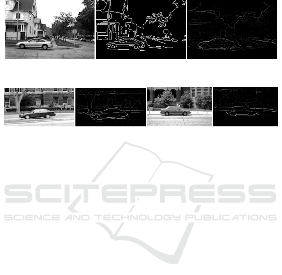
(a) (b) (c)
Figure 1: (a) Input image (b) Canny edge image (low thresh.: 0.6; high thresh.: 0.9) (c) Edge output of Structured Edge
Detector (trained for car edge detection + sharpening).
(a) (b) (c) (d)
Figure 2: (a) Input image (b) Output of Structured Edge Detector (c) Input image (d) Output of Structured Edge Detector
(both trained for car edge detection + sharpening).
efficiency (see Figure 1b). In the context of the GHT
/ DGHT, this leads to impressive object localization
performance on a large variety of tasks with limited
target object variability (Ecabert and Thiran, 2004;
Ruppertshofen et al., 2010). However, in many object
recognition tasks the images are often characterized
by a highly variable background composed of many
confounding objects and structures, clutter etc. (see
e.g. Figures 1 - 3). In those cases, the Canny Edge
Detection leads to many unwanted edges which cast
votes in addition to the required edge pixels of the
target object (Figure 1b). Thus, the voting pattern
may be significantly perturbed, potentially leading to
a mislocalization.
Recently, an improved edge detection algorithm
has been proposed (Doll
´
ar and Zitnick, 2013). The
main idea is to learn from training data the appearance
of target object edge pixels in order to discriminate
them from the edge pixels of all other structures. In
this way, confusing edges can be suppressed, so that
the target object(s) in the image are better pronounced
(see Figures 1c and 2). Thus, this technique poten-
tially avoids the generation of many Hough space
votes which do not arise from the target object and
may therefore substantially improve the localization
performance.
In this work, we compare the Structured Edge De-
tector (Doll
´
ar and Zitnick, 2013; Doll
´
ar and Zitnick,
2014) to a standard Canny Edge Detector in the con-
text of DGHT-based automatic object localization. In
particular, we quantitatively analyze the object local-
ization performance with the two edge detectors in
two real-world tasks, namely pedestrian and car local-
ization. We obtain significant performance improve-
ments on both tasks when using the Structured Edge
Detector, as compared to Canny Edge Detection. The
results demonstrate that the GHT / DGHT framework
can be successfully applied to automatic object lo-
calization scenarios with a large degree of variability
with respect to background and clutter.
The rest of the paper is organized as follows: The
Canny Edge Detection and the Structured Edge De-
tection algorithms are briefly summarized in Section
2, followed by a short presentation of the DGHT ob-
ject localization approach. The databases used in our
study, experimental results and analyses are reported
in Section 3. A discussion and conclusion can be
found in Sections 4 and 5.
2 METHODS
2.1 Edge Detection
2.1.1 Canny Edge Detection
In 1986 John Francis Canny introduced a general and
robust approach for edge detection in images (Canny,
1986). The values of the first derivatives in horizontal
and vertical direction, G
x
and G
y
, are obtained by ap-
plying the Sobel operator to the input image smoothed
with a Gaussian filter to reduce noise. Using these
values, the gradient magnitude and the edge direction
can be calculated:
VISAPP 2016 - International Conference on Computer Vision Theory and Applications
394
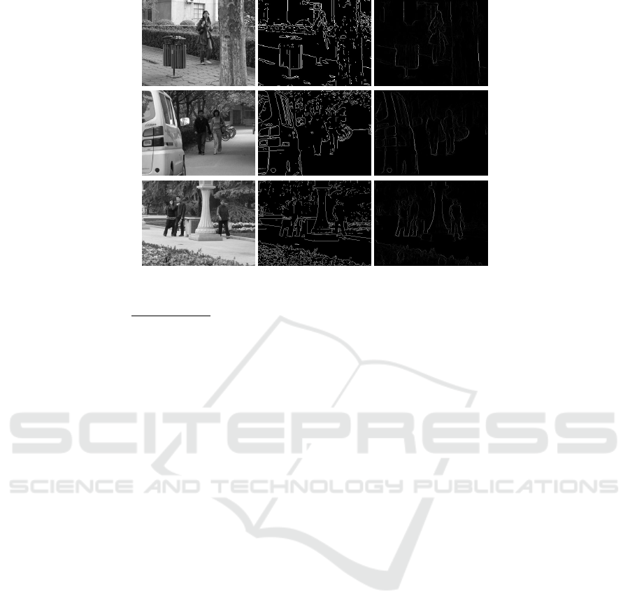
Figure 3: Examples of confusing Canny edges and background clutter in pedestrian localization.
(Left) Input image (middle) Canny edge image (right) Output of Structured Edge Detector (trained for ped. edge detection).
G =
q
(G
x
)
2
+ (G
y
)
2
(1)
θ = arctan(G
y
,G
x
) (2)
The resulting edges are thinned using non-
maximum suppression (NMS). Subsequently, the re-
maining edge pixels are classified using a high and a
low threshold value. Edges above the high threshold
(strong edges) are kept, whilst edges below the low
threshold are discarded. Edges between the low and
the high threshold are so called weak edges. Whether
they will remain in the resulting edge image is de-
termined by hysteresis, i.e. those edges are kept
only if there is a strong edge within the respective 8-
connected neighborhood. Examples of Canny edge
images are provided in Figures 1b and 3.
Other variants of edge detection based on first or
second order derivatives exist, see e.g. (Shrivakshan
and Chandrasekar, 2012) or anisotropic Gaussian fil-
tering (Knossow et al., 2007; Montesinos and Mag-
nier, 2010). Their evaluation is however beyond the
scope of this work.
2.1.2 Structured Edge Detection
Recently, Doll
´
ar and Zitnick introduced a novel ma-
chine learning approach for detecting edges, which
incorporates information on the object of interest
(Doll
´
ar and Zitnick, 2013; Doll
´
ar and Zitnick, 2014).
Their approach utilizes the fact that patches of edges
show common forms of local structure like straight
lines or T-junctions or similar (Doll
´
ar and Zitnick,
2014). Thus, a learning framework, like Random
Forests, can be applied to assign an output edge
patch to features extracted from an input image patch.
As features, Doll
´
ar and Zitnick use pixel-lookups
and pairwise-difference features of 13 channels (three
color, two magnitude and eight orientation feature
channels). However, since the space of observed
image patches is high-dimensional and complex, it
is mapped to a discrete space based on ideas of
structured learning (Nowozin and Lampert, 2011;
Kontschieder et al., 2011), thus enabling an efficient
training of Random Forests (Breiman, 2001). For a
test image, the trained detector is applied to densely
sampled, overlapping image patches. The resulting
edge patch predictions which refer to the same image
pixel are locally averaged after applying a sharpening
procedure in order to reduce diffusion. This is done
by aligning each predicted edge patch to the underly-
ing image patch data.
Using the novel edge detection algorithm which
runs at real-time, Doll
´
ar and Zitnick obtained state-of-
the-art accuracy on two contour datasets and demon-
strated cross-dataset generalization (Doll
´
ar and Zit-
nick, 2013; Doll
´
ar and Zitnick, 2014).
2.2 Object Localization
2.2.1 Generalized Hough Transform
The Generalized Hough Transform (GHT), intro-
duced by Ballard in 1981 (Ballard, 1981), is a general
and well-known model-based approach for object lo-
calization, which belongs to the category of template-
matching techniques. Each model point m
j
is repre-
sented by its coordinates with respect to the reference
point.
The GHT transforms a feature image, in our case
an edge image, into a parameter space, called Hough
space, utilizing a simple voting procedure. The
Structured Edge Detection for Improved Object Localization using the Discriminative Generalized Hough Transform
395

Hough space consists of accumulator cells (Hough
cells), representing possible target point locations
and, potentially, shape model transformations. The
number of votes per accumulator cell reflects the de-
gree of matching between the (transformed) model
and the feature image.
Since each additional parameter in a model trans-
formation directly increases the computational com-
plexity of the algorithm, we restrict the model trans-
formation to a simple translation in this work. Moder-
ate object variability with respect to shape, size, and
rotation is not explicitly parameterized, but implicitly
learned into the model by appropriately placing model
points as indicated by the training data.
The voting procedure, which transforms a feature
image X into the Hough space H (with discrete el-
ements c
i
) by using the shape model M, can be de-
scribed by
H(c
i
,X) =
∑
∀m
j
∈M
f
j
(c
i
,X) (3)
with
1
f
j
(c
i
,X) =
∑
∀e
i
∈X
1, if c
i
= b(e
i
− m
j
)/ρc
and |ϕ
e
i
− ϕ
m
j
| < ∆φ
0, otherwise.
(4)
The quantized Hough space H (with quantization
parameter ρ) consists of Hough cells c
i
that accumu-
late the number of matching pairs of all model points
m
j
and feature points e
i
. Each Hough cell c
i
repre-
sents a target hypothesis whose coordinates in image
space are given by b(c
i
+ 0.5) · ρc.
f
j
(c
i
,X) determines how often model point m
j
votes for Hough cell c
i
for the given feature image
X. However, note that a voting is only possible, if
the orientation
2
of the model and feature point, ϕ
m
j
and ϕ
e
i
, respectively, has a small difference of below
∆φ. The most likely target point location results from
the Hough cell ˜c(X) with the highest number of votes,
corresponding to the best match between the model M
and the feature image X:
˜c(X) = argmax
c
i
H(c
i
,X) (5)
2.2.2 Discriminative Generalized Hough
Transform
The Discriminative Generalized Hough Transform
(DGHT) extends the Generalized Hough Transform
(Section 2.2.1) by an individual weighting scheme for
1
Note that bac denotes the floor of each component of a.
2
I.e. the gradient direction as in Eq. 2
the J model points m
j
of the shape model M, opti-
mized by a discriminative training algorithm.
During the voting procedure of Equation 3, the in-
dividual model point weights λ
j
are incorporated as
described in Equation 6:
H(c
i
,X) =
∑
∀m
j
∈M
λ
j
f
j
(c
i
,X) (6)
with f
j
(c
i
,X) as in Equation 4.
In GHT-based approaches, the quality of the local-
ization highly depends on the quality of the model. A
good model has to fulfill two important conditions: A
high correlation with the feature image on the target
point location and a small correlation at confusable
objects. In the DGHT, this is achieved by an iterative
training procedure. It starts with an initial model that
is generated by superimposing annotated feature im-
ages at the reference point. The model point weights
λ
j
are optimized using a Minimum Classification Er-
ror (MCE) approach, and model points with a low
absolute weight are eliminated. At last, the model
is extended by target structures from training images
which still have a high localization error. This pro-
cedure is repeated until all training images are used
or have a low localization error. A more detailed
description of the technique can be found in (Rup-
pertshofen, 2013).
2.2.3 Shape Consistency Measure
As a result of the iterative training procedure (see Sec-
tion 2.2.2), the DGHT models may cover medium ob-
ject variability (e.g. regarding size, aspect) by con-
taining model points representing the most important
modes of variation observed in the training data. In
the GHT / DGHT voting procedures (Eqs. 3 and 6, re-
spectively), it can be seen that these points vote inde-
pendently for a localization hypothesis c
i
. This means
that f
j
(c
i
,X) is not influenced by f
k
(c
i
,X),∀ j 6= k. In
practice, however, these dependencies exist since mu-
tually exclusive variations should not be allowed to
accumulate their votes for the same Hough cell c
i
. For
example, a subset of the model points may represent
a frontal view of a person, and a different subset a
side view of a person. While it is reasonable to in-
corporate aspect variations into the Hough model, the
voting of model points from mutually exclusive varia-
tion types should not be mixed. This is, since a Hough
cell might coincidentally get a large number of votes
from different variants which may lead to a mislocal-
ization.
To this end, (Hahmann et al., 2015) suggested to
analyse the pattern of model points voting for a par-
ticular Hough cell c
i
. More specifically, this model
VISAPP 2016 - International Conference on Computer Vision Theory and Applications
396

(a)
(b)
Figure 4: Sample images of (a) UIUC Car Database and (b) subset of IAIR-CarPed.
point pattern is classified into a class ”regular shape”
Ω
r
(representing e.g. frontal view of a person or a
side view of a person) and a class ”irregular shape”
Ω
i
. Note that the exact number of votes from a model
point m
j
for a particular cell c
i
is less relevant than
the distance d(c
i
,c
k
) between cell c
i
and the closest
cell c
k
in the neighborhood of c
i
for which the model
point m
j
voted for. Therefore, the attribute vector
R(c
i
,X) = {r
1
(c
i
,X),r
2
(c
i
,X),..., r
J
(c
i
,X)} (7)
is introduced with
r
j
(c
i
,X) = min
c
k
d(c
i
,c
k
), if f
j
(c
k
,X) ≥ 1
and d(c
i
,c
k
) < ϑ
ϑ, otherwise
(8)
and d(a,b) = max
t
|a
t
− b
t
|. A value α =
r
j
(c
i
,X) < ϑ indicates that the model point m
j
voted
in a (2α + 1)× (2α + 1) neighborhood around c
i
. The
parameter ϑ serves as a maximum limit up to which
a relation from model point m
j
to Hough cell c
i
can
be assumed. Above this (experimentally optimized)
limit of seven cells a link between m
j
and c
i
is un-
likely and therefore the exact distance is irrelevant for
the analysis of the voting pattern. The attribute vector
R(c
i
,X) is used as input for a Random Forest Classi-
fier, which is trained on appropriate training data to
discriminate the two classes. For a test image X, a
(D)GHT model is applied to generate a Hough space
H(c
i
,X) and a list of most probable object positions c
i
(which correspond to an ordered list of the positions
of the maxima in Hough space). For each candidate
c
i
, the attribute vector R(c
i
,X) is calculated from Eqs.
7 and 8, and the Random Forest Classifier is used to
calculate the probability p(Ω
r
|R(c
i
,X)) that the set of
model points, voting for c
i
, has a regular shape.
The obtained probability is used in the localiza-
tion procedure as an additional weighting factor for
the Hough space votes, changing Eq. 5 to
˜c(X) = argmax
c
i
p(Ω
r
|R(c
i
,X)) · H(c
i
|X) (9)
We refer to the Random Forest classification of the
Hough voting pattern, Eq. 9, as Shape Consistency
Measure (SCM). To generate the required attribute
vectors for the training of the Random Forest Clas-
sifier, the DGHT is applied to each training image.
Then the class labels Ω
r
and Ω
i
are assigned to the
individual Hough cells of the training images using
the following rule: Cells with a localization error be-
low a threshold ε
1
are labelled as class Ω
r
while those
with an error of above ε
2
are assigned to class Ω
i
. Hy-
potheses which cannot be assigned to either class are
not used in the Random Forest training in order to en-
sure a better discrimination between the two classes.
3 EXPERIMENTS
3.1 Databases
In this work, we apply our object localization frame-
work (consisting of DGHT and SCM, Eq. 9) to two
kinds of feature images: Edge images generated by
applying the Canny Edge Detector (Section 2.1.1) and
the Structured Edge Detector (Section 2.1.2). In par-
ticular, we evaluate the performance of the Canny and
Structured Edge Detector as features for the DGHT
on two datasets:
The first one is the UIUC Car Database (Agarwal
and Roth, 2002; Agarwal et al., 2004). Here, we use
the 550 positive car training images for model train-
ing, all 1050 training images (550 positive and 500
negative) for the training of the Shape Consistency
Measure and the 170 single-scale test images for per-
formance evaluation.
The second database, used for pedestrian localiza-
tion, is a subset of the IAIR-CarPed database (Wu
et al., 2012). We filtered the dataset for images con-
taining pedestrians and computed the mean height
(150 px). In order to include size variability to a
moderate extent, we decided for a pedestrian height
range of approximately 25% of the mean height. This
leads to a pedestrian height range of 130 to 170 pixels.
We keep all images containing pedestrians of a size
Structured Edge Detection for Improved Object Localization using the Discriminative Generalized Hough Transform
397

within this range and discard images containing only
smaller ones. Images with larger pedestrians were
downscaled by a random factor such that the scaled
pedestrian height falls into the specified range. Fol-
lowing this procedure we obtain 457 images, of which
the first 300 were used to train the DGHT model and
the SCM and the remaining 157 images were used for
evaluation. In the test set only pedestrians within the
size range remain annotated.
Sample images of both datasets are shown in Fig-
ure 4.
3.2 Experimental Setup and System
Parameters
As a first edge detector, we use the Canny Edge De-
tector. Here, we specifically optimize the low and
high threshold for each localization task. This is done
by qualitatively assessing the Canny edge images on a
sample basis, searching for a tradeoff between keep-
ing essential edges of the target object and not hav-
ing too much background clutter. For the UIUC Car
Database we use a high threshold percentage of 0.9
and a low threshold percentage of 0.6. For the pedes-
trian localization task on the IAIR-CarPed subset we
use a high threshold percentage of 0.8 and a low
threshold percentage of 0.5.
As a second edge detector, we use the Structured
Edge Detector from Doll
´
ar and Zitnick. For com-
puting the structured edges we use publicly avail-
able code
3
. As explained in Section 2.1.2, the Struc-
tured Edge Detector must be trained with domain-
specific, annotated edge images. In our case, we use
the cars side category of Caltech-101 database (Fei-
Fei et al., 2006) and the PennFudan dataset (Wang
et al., 2007) for cars and pedestrians, respectively
4
.
In this manner, the specific Structured Edge Detec-
tors are trained to highlight edges belonging to the
respective object category and suppress background
edges or those of non-target objects. We refer to the
domain-specific Structured Edge Detector as SSE.
For comparison, we also used a general purpose
Structured Edge Detector provided by Doll
´
ar and
Zitnick. This edge detector is trained on the gen-
eral BSDS500 segmentation dataset (Arbelaez et al.,
2011) and is referred to as GSE.
The experiments for the different edge images on
both datasets are conducted as follows:
3
http://research.microsoft.com/en - us/downloads/38910
9f6-b4e8-404c-84bf-239f7cbf4e3d, accessed: 2015-09-16
4
We use these databases and not UIUC and IAIR for the
training of the specific structured edge detectors, because
the former already provide a ground truth contour annota-
tion.
First, the different feature images (Canny, GSE
and SSE) are generated for both datasets, which serve
as input images for the DGHT training. Then, a
DGHT model is trained for each feature type and
dataset using the iterative training process according
to Section 2.2.2. The quantization parameter ρ is set
to 2 in x- and y-direction and ∆Φ to 16 for all experi-
ments. Afterwards, the Shape Consistency Measure
(SCM) is trained by applying the resulting DGHT
model to each training image and extracting local-
ization hypotheses below ε
1
5
as samples for Ω
r
and
above ε
2
6
as samples for Ω
i
(see Section 2.2.3) with
ϑ set to 7. After these training steps both the DGHT
model and the SCM are applied to the test image set,
where the same edge detection algorithm as in train-
ing is applied to each test image. Then, for each test
image X we compute the best localization hypothesis
˜c
i
(X) according to Eq. 9.
3.3 Results
In order to classify whether the best localization hy-
pothesis ˜c
i
(X) per image X is a correct localization,
we use the common PASCAL VOC overlap measure
(Everingham et al., 2010):
a
0
=
area(B
p
∩ B
gt
)
area(B
p
∪ B
gt
)
, (10)
where B
p
∩ B
gt
refers to the intersection and B
p
∪ B
gt
to the union of the predicted bounding box B
p
and the
ground truth bounding box B
gt
. For a correct detec-
tion the overlap measure a
0
must exceed 0.5.
Because this measure needs a predicted bounding
box, we need to obtain B
p
from the best localization
hypothesis ˜c
i
(X). In the UIUC single-scale test set,
we take the fixed object width and height as the width
and height of B
p
around ˜c
i
(X) as the center point.
For pedestrian localization in the size range of 130 to
170 px, we take the mean object width and height as
the width and height of B
p
around ˜c
i
(X) as the center
point.
The localization and detection results for the
UIUC single-scale test set and for the test subset of
IAIR-CarPed are shown in Table 1 and 2, respec-
tively. A bar chart of the localization accuracies on
both datasets with the investigated edge detection al-
gorithms is presented in Figure 6. Since multi-object
detection is currently not being addressed in our local-
ization framework, please note that all reported results
are with respect to the overlap score a
0
of the best hy-
pothesis ˜c
i
(X) with respect to the closest ground truth
5
5 and 10 for UIUC and IAIR, respectively.
6
15 and 25 for UIUC and IAIR, respectively.
VISAPP 2016 - International Conference on Computer Vision Theory and Applications
398
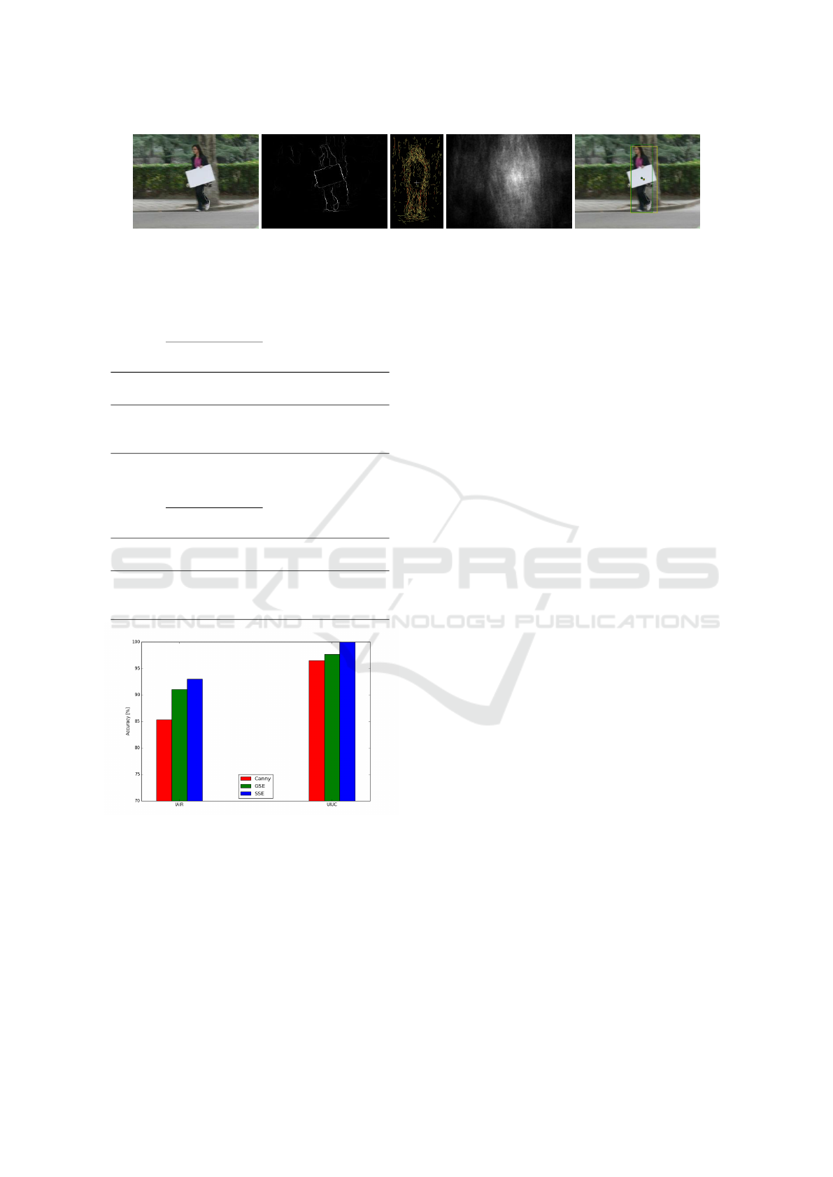
(a) (b) (c) (d) (e)
Figure 5: Sample localization with: (a) Input image (b) Structured Edge Detection output (c) Learned model for pedestrian
detection (d) Hough space (e) Resulting localization; yellow: prediction, green: ground truth annotation.
Table 1: Localization results on UIUC single-scale.
Accuracy:
# of images with a
0
>0.5
total # of images
; Localization error: dis-
tance of ˜c
i
(X) to closest ground truth annotation in pixel.
Feature Accuracy Mean a
0
Mean loc.
[%] [%] error [px]
Canny 96.47 77.69 4.46
GSE 97.65 79.72 4.39
SSE 100.00 82.83 3.13
Table 2: Localization results on IAIR-CarPed subset
database.
Accuracy:
# of images with a
0
>0.5
total # of images
; Localization error: dis-
tance of ˜c
i
(X) to closest ground truth annotation in pixel.
Feature Accuracy Mean a
0
Mean loc.
[%] [%] error [px]
Canny 85.35 64.19 20.07
GSE 91.08 69.65 12.56
SSE 92.99 69.27 15.71
Figure 6: Localization accuracies of the different edge
detectors (see Section 2.1) for both databases.
annotation per test image X only. Therefore, the ac-
curacy denotes the number of images with a correct
localization, i.e. the overlap between the predicted
and the closest ground truth bounding box according
to Eq. 10 must exceed 0.5, in relation to the total
amount of test images.
4 DISCUSSION
In the car localization task on the UIUC single-scale
set, using task-specific structured edges (SSE) instead
of Canny edges improves localization accuracy from
96.47% to 100%. This is because the trained car SSE
edge detector can successfully suppress many confus-
ing edges of non-target objects as in the example in
Figure 7. Here, the maximum in Hough space inci-
dentally arising from non-object-related edges, which
is observed for Canny edges and leads to a wrong ob-
ject localization, disappears when using SSE features.
Instead, the object-related edges lead to a maximum
in Hough space at the (almost) correct object position
(see Figure 7). The accuracy of the GSE features rank
in between (97.65%). This means that without an ad-
ditional category-specific training effort the localiza-
tion accuracy compared to Canny edges can still be
improved, although less than with task-specific struc-
tured edges.
Regarding the pedestrian localization task, the
conclusions from the car localization task can be con-
firmed, however, in a harder task exhibiting size vari-
ability and much more confusable background struc-
tures (see Figure 4b). We obtained accuracy values
of 85.35% for Canny, 91.08% for GSE and 92.99%
for SSE, respectively. These numbers demonstrate
that also the pedestrian localization performance can
be substantially increased using specifically trained
SSE features. When qualitatively inspecting the error
cases of the SSE experiment, in eight of the eleven
mislocalizations, however, pedestrians were localized
(see Figure 8), but their height is not within the al-
lowed size range from 130 to 170 px (Section 3.1) and
therefore those pedestrians are not annotated leading
to an overlap a
0
of 0%. When slightly enlarging the
annotated size range to 120 to 180 px the localization
accuracies are 89.17% (Canny), 94.27% (GSE) and
95.54% (SSE), respectively.
To assess the statistical significance of the accu-
racy, we assume a binomial distribution for the de-
tection results per image (correctly localized versus
not correctly localized, corresponding to a
0
> 0.5 ver-
Structured Edge Detection for Improved Object Localization using the Discriminative Generalized Hough Transform
399

Figure 7: Example feature images and localization results on UIUC (rows 1 - 4) and IAIR (rows 5 - 8);
Odd rows: Canny Edge Detection, even rows: Structured Edge Detection (SSE)
(First column) Input image (Second column) Edge image (Third column) Hough space (Fourth column) Localization
result; yellow: prediction, green: ground truth annotation. (Best viewed in color).
sus a
0
<= 0.5, respectively), and calculate the 95%-
Clopper-Pearson confidence interval for the accuracy
(see Table 3). On both tasks, the localization accu-
racy of the SSE edges is beyond the confidence inter-
val for the localization accuracy using Canny edges,
demonstrating a significant improvement in localiza-
tion accuracy by structured edges compared to Canny
edges. On the pedestrian localization task, this also
holds when using GSE edges.
To assess statistical significance of the continuous
overlap parameter a
0
when using category-specific
structured edges as input features, we use the non-
parametric Wilcoxon-Mann-Whitney test (Wilcoxon,
1945; Mann and Whitney, 1947), since a
0
is not nor-
VISAPP 2016 - International Conference on Computer Vision Theory and Applications
400
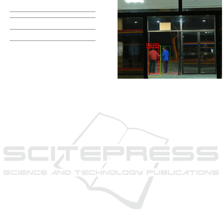
Table 3: Clopper-Pearson intervals for the experiment re-
sults.
Dataset Feature CP Interval
UIUC Canny [92.48%, 98.69%]
SSE [97.85%, 100.0%]
IAIR Canny [78.83%, 90.48%]
SSE [87.81%, 96.45%]
mally distributed (p-values of all experiments in the
Shapiro-Wilk tests (Shapiro and Wilk, 1965) are <
10e-3). Comparing the independent groups Canny
and SSE for both datasets in the Wilcoxon-Mann-
Whitney test, we obtain p-values of 9.86e − 6 and
0.001872 for UIUC and IAIR, respectively. Thus,
the mean overlap value a
0
for the SSE edge detec-
tion tests is larger at the 95% confidence level than
the mean overlap for the Canny Edge Detection tests.
Additionally, we statistically evaluated the result-
ing localization errors for Canny and SSE edge fea-
tures in the same way as described above. We obtain
p-values of 0.005118 and 0.001696 for UIUC and
IAIR, respectively. Therefore, the mean localization
error for the SSE edge detection tests is lower at the
95% confidence level than the mean localization error
for the Canny Edge Detection tests.
5 CONCLUSIONS
We have shown that the object localization perfor-
mance obtained by the voting-based DGHT approach
in real-world tasks with variable background and clut-
ter can be significantly improved by a sophisticated
edge detection algorithm, namely the Structured Edge
Detector. This applies to general structured edge
features without additional training effort as well as
category-specific Structured Edge Detectors in par-
ticular. More precisely, we obtained absolute im-
provements in localization accuracy of 3.53% and
7.64% on a car and pedestrian localization task, re-
spectively. We conclude that the DGHT framework
can be successfully used for object localization also
in real-world images with larger and more variable
background.
In future work, we aim to integrate an intelligent
edge detection mechanism into the voting framework
and to explore strategies to handle object variability
(e.g. object size, rotation) as well as multi-object and
multi-class localization.
Figure 8: Error case: Detected pedestrian is not within the
annotated height range of 130-170 px. Bounding box col-
ors: yellow: prediction; green: ground truth annotation;
red: not in ground truth, because height 6∈ [130,170] px.
(Best viewed in color).
REFERENCES
Agarwal, S., Awan, A., and Roth, D. (2004). Learning to
detect objects in images via a sparse, part-based rep-
resentation. IEEE Transactions on Pattern Analysis
and Machine Intelligence, 26(11):1475–1490.
Agarwal, S. and Roth, D. (2002). Learning a sparse repre-
sentation for object detection. In Computer Vision –
ECCV 2002, pages 113–127. Springer.
Andriluka, M., Roth, S., and Schiele, B. (2008).
People-tracking-by-detection and people-detection-
by-tracking. In IEEE Conference on Computer Vision
and Pattern Recognition, pages 1–8. IEEE.
Arbelaez, P., Maire, M., Fowlkes, C., and Malik, J. (2011).
Contour detection and hierarchical image segmenta-
tion. IEEE Transactions on Pattern Analysis and Ma-
chine Intelligence, 33(5):898–916.
Ballard, D. H. (1981). Generalizing the hough trans-
form to detect arbitrary shapes. Pattern recognition,
13(2):111–122.
Breiman, L. (2001). Random forests. Machine learning,
45(1):5–32.
Canny, J. (1986). A computational approach to edge de-
tection. IEEE Transactions on Pattern Analysis and
Machine Intelligence, (6):679–698.
Chaohui, Z., Xiaohui, D., Shuoyu, X., Zheng, S., and Min,
L. (2007). An improved moving object detection al-
gorithm based on frame difference and edge detec-
tion. In Fourth International Conference on Image
and Graphics, pages 519–523. IEEE.
Doll
´
ar, P. and Zitnick, C. L. (2013). Structured forests for
fast edge detection. In IEEE International Conference
on Computer Vision, pages 1841–1848. IEEE.
Doll
´
ar, P. and Zitnick, C. L. (2014). Fast edge detection
using structured forests.
Ecabert, O., Peters, J., Schramm, H., Lorenz, C., Von Berg,
J., Walker, M. J., Vembar, M., Olszewski, M. E., Sub-
ramanyan, K., Lavi, G., et al. (2008). Automatic
Structured Edge Detection for Improved Object Localization using the Discriminative Generalized Hough Transform
401

model-based segmentation of the heart in ct images.
IEEE Transactions on Medical Imaging, 27(9):1189–
1201.
Ecabert, O. and Thiran, J.-P. (2004). Adaptive hough trans-
form for the detection of natural shapes under weak
affine transformations. Pattern Recognition Letters,
25(12):1411–1419.
Everingham, M., Van Gool, L., Williams, C. K., Winn, J.,
and Zisserman, A. (2010). The pascal visual object
classes (voc) challenge. International journal of com-
puter vision, 88(2):303–338.
Fei-Fei, L., Fergus, R., and Perona, P. (2006). One-
shot learning of object categories. IEEE Transac-
tions on Pattern Analysis and Machine Intelligence,
28(4):594–611.
Gavrila, D. M. (2000). Pedestrian detection from a moving
vehicle. In Computer Vision – ECCV 2000, pages 37–
49. Springer.
Hahmann, F., B
¨
oer, G., Deserno, T. M., and Schramm,
H. (2014). Epiphyses localization for bone age as-
sessment using the discriminative generalized hough
transform. In Bildverarbeitung f
¨
ur die Medizin, pages
66–71. Springer.
Hahmann, F., B
¨
oer, G., Gabriel, E., Meyer, C., and
Schramm, H. (2015). A shape consistency measure
for improving the generalized hough transform. In
10th Int. Conf. on Computer Vision Theory and Ap-
plications, VISAPP.
Hahmann, F., Ruppertshofen, H., B
¨
oer, G., Stannarius,
R., and Schramm, H. (2012). Eye localization us-
ing the discriminative generalized Hough transform.
Springer.
Knossow, D., Van De Weijer, J., Horaud, R., and Ron-
fard, R. (2007). Articulated-body tracking through
anisotropic edge detection. In Dynamical Vision,
pages 86–99. Springer.
Kontschieder, P., Rota Bul
´
o, S., Bischof, H., and Pelillo, M.
(2011). Structured class-labels in random forests for
semantic image labelling. In IEEE International Con-
ference on Computer Vision, pages 2190–2197. IEEE.
Mann, H. B. and Whitney, D. R. (1947). On a test of
whether one of two random variables is stochastically
larger than the other. The annals of mathematical
statistics, pages 50–60.
Montesinos, P. and Magnier, B. (2010). A new percep-
tual edge detector in color images. In Advanced Con-
cepts for Intelligent Vision Systems, pages 209–220.
Springer.
Nowozin, S. and Lampert, C. H. (2011). Structured learn-
ing and prediction in computer vision. Foundations
and Trends
R
in Computer Graphics and Vision, 6(3–
4):185–365.
Ruppertshofen, H. (2013). Automatic modeling of anatom-
ical variability for object localization in medical im-
ages. BoD – Books on Demand.
Ruppertshofen, H., Lorenz, C., Beyerlein, P., Salah, Z.,
Rose, G., and Schramm, H. (2010). Fully automatic
model creation for object localization utilizing the
generalized hough transform. In Bildverarbeitung f
¨
ur
die Medizin, pages 281–285.
Shapiro, S. S. and Wilk, M. B. (1965). An analysis
of variance test for normality (complete samples).
Biometrika, pages 591–611.
Shrivakshan, G. and Chandrasekar, C. (2012). A compari-
son of various edge detection techniques used in im-
age processing. IJCSI International Journal of Com-
puter Science Issues, 9(5):272–276.
Wang, L., Shi, J., Song, G., and Shen, I.-F. (2007). Ob-
ject detection combining recognition and segmenta-
tion. In Computer Vision – ACCV 2007, pages 189–
199. Springer.
Wilcoxon, F. (1945). Individual comparisons by ranking
methods. Biometrics bulletin, pages 80–83.
Wu, Y., Liu, Y., Yuan, Z., and Zheng, N. (2012). Iair-
carped: A psychophysically annotated dataset with
fine-grained and layered semantic labels for object
recognition. Pattern Recognition Letters, 33(2):218–
226.
VISAPP 2016 - International Conference on Computer Vision Theory and Applications
402
