
Simultaneous Surface Segmentation and BRDF Estimation
via Bayesian Methods
Malte Lenoch, Thorsten Wilhelm and Christian W
¨
ohler
Image Analysis Group, TU Dortmund University, Otto-Hahn-Strasse 4, Dortmund, Germany
Keywords:
Image Segmentation, BRDF Estimation, Reversible Jump Markov Chain Monte Carlo.
Abstract:
We present a novel procedure that achieves segmentation of an arbitrary surface relying on the maximum
a-posteriori estimation of its reflectance parameters. The number of surfaces segments is computed by the
algorithm without user intervention. We employ Markov Chain Monte Carlo algorithms to compute the prob-
ability distributions associated with the model parameters of a Blinn reflectance model based on the input
images. The fact that parameters are treated as probability distributions enables us to directly draw addi-
tional information about the certainty of the estimation from the results of both parameters and segmentation
borders. Reversible jump MCMC allows us to include an unspecified number of change points in the computa-
tion, such that the algorithm explores model and parameter space at the same time and derives a segmentation
of the surface from the input data. To accomplish this, we extend the existing concept of change points to
two dimensions introducing a number of necessary new regulations and properties. The performance of the
segmentation and reflectance estimation is evaluated on a synthetic and a real-world dataset.
1 INTRODUCTION
Many man-made objects or natural materials exhibit
a reflectance that is non-uniform across the surface.
The estimation of a spatially varying bi-directional
reflectance distribution function (SVBRDF) is a well-
approached research task in computer vision as well
as in photogrammetric backgrounds. Additionally, it
is of interest in certain tasks, to determine the surface
areas that consist of the same material and are there-
fore associated with identical reflectance properties.
Our goal is to segment the surface of an arbitrary
object into meaningful regions based on the reflection
properties of those particular regions. We apply meth-
ods from Bayesian statistics to compute the posterior
of the acquired BRDF parameters and the patch bor-
ders based on the given input data and the specified
prior distributions, reflecting knowledge which is at
hand prior to the experiment. Since we handle every
parameter as a stochastic distribution, we know the
uncertainty of the estimate as well, instead of only
handling a point estimate as do common gradient de-
scent procedures. Furthermore, confidence analysis
in classical statistics is inferred from asymptotic the-
ory assuming large datasets, which simply does not
always hold in practice, e.g. (King et al., 2010). The
combination of Bayesian statistics and reflectance es-
timation has had little attention in recent years.
In our approach, we focus on patchwise BRDF ac-
quisition that ensures sufficient data even when not
many input images are available. The estimation of
pixelwise BRDF parameters requires a large amount
of data to be available at every surface point to reli-
ably fit the desired BRDF model, e.g. (Lensch et al.,
2003; Goldman et al., 2005). In fact, a dense angular
representation is necessary to capture narrow specular
lobes and prevent aliasing. Due to shadowing effects,
a complex surface structure can reduce the available
intensity information per pixel to be smaller than the
number of captured images. We assume isotropic re-
flectance and neglect the influence of subsurface scat-
tering or translucency.
2 RELATED WORK
The scope of BRDF reproduction in previous work
ranges from the acquisition of pure albedo informa-
tion to the reconstruction of per-pixel sets of param-
eters of complex BRDF models, e.g. Weyrich et al.
(2008); Aittala et al. (2013).
A common approach to estimate the SVBRDF of
an unknown material is to compute mixture maps as-
Lenoch, M., Wilhelm, T. and Wöhler, C.
Simultaneous Surface Segmentation and BRDF Estimation via Bayesian Methods.
DOI: 10.5220/0005722600390048
In Proceedings of the 11th Joint Conference on Computer Vision, Imaging and Computer Graphics Theory and Applications (VISIGRAPP 2016) - Volume 4: VISAPP, pages 39-48
ISBN: 978-989-758-175-5
Copyright
c
2016 by SCITEPRESS – Science and Technology Publications, Lda. All rights reserved
39

suming weighted sums of base materials to construct
an approximation of the measured intensity Gold-
man et al. (2005); Alldrin et al. (2008); Lenoch et al.
(2014). These base materials are either taken from
densely acquired datasets, e.g. the MERL database
Matusik et al. (2003), or composed of few analyti-
cal BRDF models. In the latter case, the set θ
θ
θ of pa-
rameters of the model function has to be estimated.
Goldman et al. (2005) assume two base materials per
surface and represent those with a mixture of two
Ward-BRDFs. Similarly, Lensch et al. (2003) cap-
ture reflectance samples that yield salient information
and apply mixtures of up to five Lafortune BRDFs to
clustered lumitexels. This yields more possibilities in
the model space, but requires the estimation of multi-
ple sets of parameters and a mixture map at the same
time.
The combination of BRDF estimation and prob-
abilistic methods is very rare in literature. Aittala
et al. (2013) represent reflectance that may vary along
the surface by a Gaussian mixture model in the fre-
quency domain. The initial solution is improved
with a maximum a-posteriori estimation. Louw and
Nicolls (2010) use a Markov random field to imitate
the reflectance behavior of a surface. The MRF is es-
timated with a Population Markov Chain Monte Carlo
algorithm Laskey and Myers (2003).
3 PROPOSED PROCEDURE
The BRDF fitting procedure requires the illumina-
tion geometry to be known. This can be ensured
easily, if 3D information about the surface is avail-
able. However, the approach works independent of
the source of the 3D data and could be integrated in
a self-consistent algorithm similar e.g. to Herbort and
W
¨
ohler (2012), that has no prior knowledge about the
surface shape.
3.1 Bayesian BRDF Modeling
We choose the BRDF model according to Blinn
(1977) in the physically plausible modification by
Giesen (2009) combined with a Lambertian term
(Lambert, 1760) to account for diffuse reflection.
We assume that this relatively simple model suffices,
since the unknown surface will be segmented during
the procedure and complex reflectance can be mod-
eled by small segments of different parameters. Note
that we do not require physical materials to coincide
with segmented patches, since even within the same
material subtle changes can require changing BRDF
parameters to achieve accurate modeling.
In terms of Bayesian statistics, the BRDF model
is the mean of a normal distributed likelihood. We
assume the residuals of the BRDF model to follow a
Gaussian distribution with an unknown variance σ
2
.
Since σ
2
is unknown, we estimate it as a part of the
procedure and are thus able to quantify the deviation
of the model from the observed data which based on
the BRDF model formulation by Giesen (2009) leads
to
y
y
y ∼ N (µ
µ
µ, σ
2
) (1)
µ
µ
µ =
I
0
r
2
k
d
π
+ k
s
(γ + 2)(γ + 4)
8π(2
−
γ
2
+ γ)
·
h
h · n
i
γ
h
l · n
i
(2)
1 = k
d
+ k
s
. (3)
Here
h
l · n
i
= cos∠(l
l
l, n
n
n) denotes the vector prod-
uct between the normalized vectors l
l
l and n
n
n, with sur-
face normal n
n
n, direction l
l
l of incident light, viewing
direction v
v
v and half-way vector h
h
h =
l
l
l+v
v
v
||l
l
l+v
v
v||
2
.
The chosen model thus depends on four parame-
ters. Light source intensity I
0
, diffuse and specular
weight k
d
(since k
s
= 1 − k
d
), cosine lobe exponent γ
and variance σ
2
. Each of these parameters requires
a prior to define the distribution of the parameter be-
fore any data was seen. We assume the priors to be
normal distributions; exemplarily for the light source
intensity
p(I
0
) ∼ N (µ
I
0
, σ
2
I
0
) (4)
The prior yields the possibility to involve certain
knowledge about the possible range of the parameters
into the estimation process. This fact can be exploited
if, for example, a coarse estimate of the light source
intensity exists. Yet, this estimate might be prone to
simplification errors. If there is no prior knowledge
available or only at a high level of uncertainty, a large
variance is used to reduce the influence of the prior,
since its probability is equal in almost the entire pa-
rameter space. In a Bayesian framework this is termed
an uninformative prior. A uniform distribution would
cancel out the effect of the prior completely.
Concluding from Bayes’ law we can now compute
the probability distribution of the set θ
θ
θ of model pa-
rameters for the input intensity data Y
Y
Y and the a-priori
probability p(θ
θ
θ).
p(θ
θ
θ|Y
Y
Y ) =
p(Y
Y
Y |θ
θ
θ) · p(θ
θ
θ)
p(Y
Y
Y )
(5)
The normalization factor p(Y
Y
Y ) is difficult to esti-
mate and can be omitted, since it is constant as long
as the input data does not change. Therefore the
posterior-density can be expressed as
p(θ
θ
θ|Y
Y
Y ) ∝ p(Y
Y
Y |θ
θ
θ) · p(θ
θ
θ) (6)
All information required to determine the proba-
bility distribution of the set of model parameters for
VISAPP 2016 - International Conference on Computer Vision Theory and Applications
40

the given input data is the likelihood and the prior,
which is both at hand.
3.2 Markov Chain Monte Carlo
Actually, the chosen priors can be based on additional
available information or be completely uninformative,
in any case the real distribution of θ
θ
θ remains unknown
and subject to the estimation. Markov chain Monte
Carlo (MCMC) methods as e.g. introduced by Nt-
zoufras (2011) can be employed to sample the model
parameters’ unknown distribution. To achieve this, a
Markov chain is constructed whose stationary distri-
bution corresponds to the desired unknown distribu-
tion. Thus, after a converging time, the state of the
chain can be used sample the unknown posterior.
More specifically, we use the Metropolis-Hastings
(MH) algorithm introduced by Metropolis et al.
(1953) and Hastings (1970). Accordingly, we con-
struct a Markov chain which proposes in each step
new values of the chain for the respective BRDF pa-
rameters. The likelihood of the values is assessed with
the newly generated values and if the likelihood of the
parameters increases they are probably accepted as a
new value of the chain, if not they are probably dis-
carded. The term probably refers to the acceptance
probability α that is compared to a random number,
such that there is a possibility to accept a new value
even if the likelihood decreased and vice-versa. Sim-
ilar to the priors, starting values θ
θ
θ
(0)
have to be sup-
plied by the user and can bring in additional informa-
tion.
The number T of iterations of the algorithm
is taken to be fixed. A proposal distribution
p(θ
θ
θ
(t)
|θ
θ
θ
(t−1)
) and the acceptance probability α are
necessary for the generation process; given for I
0
I
(0)
0
initial value,
p(I
(t)
0
|I
(t−1)
0
) ∼ N (I
(t−1)
0
, (σ
p
I
0
)
2
) (7)
α
I
0
= min(1, A)
A =
p(y
y
y|I
(t)
0
, k
d
, γ, σ)p(I
(t)
0
)p(k
d
)p(γ)p(σ)
p(y
y
y|I
(t−1)
0
, k
d
, γ, σ)p(I
(t−1)
0
)p(k
d
)p(γ)p(σ)
!
= min
1,
p(y
y
y|I
(t)
0
, k
d
, γ, σ)p(I
(t)
0
)
p(y
y
y|I
(t−1)
0
, k
d
, γ, σ)p(I
(t−1)
0
)
!
(8)
It is assumed here that there is no interdependence
between the parameters, such that we can apply a
componentwise MH and each parameter is proposed
and accepted individually (Ntzoufras, 2011). This
yields the general advantage, that simple proposal dis-
tributions can be applied, whereas the construction of
a combined proposal distribution can require careful
design. Still, a combined proposal distribution can
yield a faster converging chain.
After a user-defined burn-in phase the chain con-
verges to the actual unknown posterior distribution if
according to Gilks et al. (1996, p.46) the following
properties are met:
• Irreducibility
• Positive Recurrency
• Aperiodicity
At the state of convergence, statistics can be com-
puted from the drawn samples. Thusly, the adap-
tion of the BRDF model to unknown data immedi-
ately yields a confidence region for each parameter
and with σ
σ
σ
2
a measure of the accuracy of the model.
3.3 Reversible Jump Markov Chain
Monte Carlo
So far we can adapt a BRDF model to unknown in-
tensity data, but the segmentation of the surface has
not yet been regarded. Image segmentation is usually
performed in a generative way (e.g. using Gaussian
Mixture Models). We use instead a discriminative ap-
proach and directly infer the boarders of the regions
from the data. Effectively, a change in surface struc-
ture or material enforces a change of the model pa-
rameters to reproduce the received impression accu-
rately.
So-called Reversible Jump Markov chain Monte
Carlo (RJMCMC) methods as described by Green
(1995) are able to explore the parameter and model
space simultaneously. That means in terms of statis-
tics, that there is a certain probability in each itera-
tion to create, delete or modify a change point τ that
separates two sets of model parameters. Using these
change points it is possible to divide unknown data
into meaningful segments.
We have extended the concept of change points to
the two-dimensional application of image segmenta-
tion, with the following new properties:
• Change points are possible both in u and v direc-
tion (referring to image coordinates).
• A change point becomes a vector of change
points, since it will affect the entire row/column
of image pixels.
• Each pixel coordinate of the change point vector
can be moved individually.
• Surface segments are constructed from the regions
where the same change points in u and v direction
coincide.
Simultaneous Surface Segmentation and BRDF Estimation via Bayesian Methods
41

We allow change points to lie outside of the image
coordinate frame, since this is a helpful property when
segment borders are not covering a complete row or
column.
A possible maximum of change points in each di-
rection has to be defined by the user. Based on these
maxima, we construct an indicator matrix that assigns
the actual regions based on the combinations of the
change points. For example, τ
max
(u) = τ
max
(v) = 3
yield the following assignment:
(1, 1) (1, 2) (1, 3)
(2, 1) (2, 2) (2, 3)
(3, 1) (3, 2) (3, 3)
ˆ=
1 4 7
2 5 8
3 6 9
(9)
Each change point itself has a statistical distribu-
tion, such that confidence intervals can be computed
directly from the data of the Markov chain. Com-
pared to other segmentation procedures this is a note-
worthy advantage, since the algorithm gives a mea-
sure for the quality of the segmentation. The change
points are assumed to follow a uniform distribution,
s.th. τ ∼ U(−1, imagesize+1), since they are allowed
to lie outside the image plane
3.3.1 A Change in Dimension
The possibility to create or delete change points cre-
ates needs of a procedure to split and merge parame-
ter sets θ
θ
θ
i
. A new region could be initialized with the
parameters of a randomly chosen neighboring region,
yet this makes it impossible to revert the step without
storing a large amount of data. A better solution is to
have a bijective transformation M
M
M which is indepen-
dent of the actual number of change points.
A random number r is drawn from the distribu-
tion q(r) = N (0, 1) and symmetrically added and
subtracted from the existing change points. In-
spired by Pascal’s triangle the coefficients P
n
(k) =
(−1)
k
n
k
, k = 0, .., n of the last column of M
M
M create a
unique transformation when jumping from dimension
n−1 to n. For the step to n = 3 and former parameters
θ
θ
θ
(t−1)
1
and θ
θ
θ
(t−1)
2
this means
θ
θ
θ
(t)
1
θ
θ
θ
(t)
2
θ
θ
θ
(t)
3
=
1 0 −1
0.5 0.5 2
0 1 −1
θ
θ
θ
(t−1)
1
θ
θ
θ
(t−1)
2
r
. (10)
Note that the transformation has to be applied
componentwise to θ
θ
θ
i
, thus the random number r can
be scaled to the dimension of the parameter. The in-
verse of M
M
M is defined and the Markov chain can be
reset to its state in the lower dimension. This can be
helpful to reduce computational time, since the chain
can continue from its former state, possibly near con-
vergence.
The proposed change in dimension is accepted
with an acceptance probability α similar to the propo-
sition of new parameters. The dimension is repre-
sented by a model number m that is determined from
the indicator matrix. For the sake of readability the
iteration index t will be omitted in what follows and
the proposed value is indicating by an apostrophe.
α(θ
θ
θ, θ
θ
θ
0
) = min(1, B),
B =
p(θ
θ
θ
0
, m
0
|X
X
X)p(m|m
0
)q(r
0
)
p(θ
θ
θ, m|X
X
X)p(m
0
|m)q(r)
∂θ
θ
θ
0
∂(θ
θ
θ, r
r
r)
(11)
p(m
0
|m) = p(m|m
0
) is the probability to change from
one model to the other, e.g. add or delete a change
point respectively and in our approach assumed to be
equal.
∂θ
θ
θ
0
∂(θ
θ
θ,r
r
r)
is the Jacobian of the partial deriva-
tives, necessary since what we do is basically a co-
ordinate transformation. Yet, the Jacobian is only a
scaling factor, which may be omitted and thus B sim-
plifies to
B =
p(θ
θ
θ
0
, m
0
|X
X
X)q(r
0
)
p(θ
θ
θ, m|X
X
X)q(r)
. (12)
The acceptance of the inverse move is simply cal-
culated as
α = min
1,
1
B
. (13)
After the predefined number of T iterations, it has
to be decided which combination of change points is
the most probable. The integration in the model space
is turned into a summation in the discrete case and the
model with the most iterations is accepted as the best
solution, e.g. (King et al., 2010). However, compar-
ing the ”time spent“ in different models yields infor-
mation about the certainty of the solution.
3.4 Synthetic Data
The algorithm is evaluated first on a synthetic dataset.
Figure 1(a) shows one of the input images and Fig-
ure 1(b) the resulting reflectance map. The similar-
ity to the result expected by the human viewer under-
lines the success of the algorithm in determining the
reflectance parameters of the surface and segmenting
its regions. The parameters of the algorithm, (σ
p
i
)
2
of
the proposal distribution, the prior parameters and the
starting values of the Markov chain θ
(0)
i
are stated in
Table 1.
The histogram of visited models is depicted in
Figure 2. The histogram counts indicate strongly that
model m = 8 is the best choice. That equals one
VISAPP 2016 - International Conference on Computer Vision Theory and Applications
42
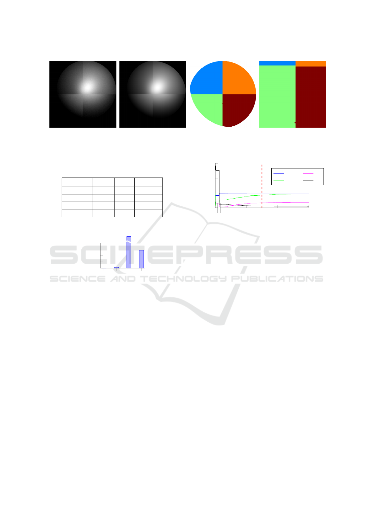
(a) (b) (c) (d)
Figure 1: (a) Exemplary input image of synthetic dataset and (b) reflectance map computed from the algorithm. Same grey
value scaling in both images. (c) Assignment of regions is almost perfect. (d) Misaligned pixel in lower right region.
Table 1: Initial values θ
(0)
i
of Markov chain, (σ
p
i
)
2
of pro-
posal distribution and prior parameters µ
prior
and (σ
prior
)
2
.
θ
(0)
i
(σ
p
i
)
2
µ
prior
(σ
prior
)
2
I
0
80 0.5 0 100
k
d
0.5 0.05 0 100
γ 1 0.07 0 100
σ
2
3 0.09 0 100
1
7
8 9
0
200
400
600
800
4
24
14,405
567
model number m
# iterations
Figure 2: Histogram of visited models in model space of
artifical dataset. Counting indicated that model 8 is the most
likely one.
change point in u and v direction and is highly consis-
tent with the dataset, as becomes apparent from Fig-
ure 1. The certainty of the algorithm is about 96%.
The sampled a-posteriori distribution of the set θ
θ
θ
of model parameters is shown along with the itera-
tions of the Markov chain in Figure 3. Convergence
of k
d
and γ is slow which may be caused by the small
(σ
p
i
)
2
of the proposal distribution (see Table 1). To
ensure that the final sampling is based on the correct
a-posteriori distribution, the burn-in phase is set to
50%, which is a conservative estimation.
To underline the efficiency of our procedure, the
inferred reflectance parameters and their uncertainties
are listed in Table 2 together with the true values that
have actually been used to generate the synthetic test
data (green values in each cell). The averages of the
parameter estimates are very similar to the actual pa-
rameter values, which is also indicated by Figure 1(a)
and (b). Moreover, the uncertainties of the estimate
0
0.5
1
1.5
·10
4
0
1
2
3
iteration t
parameter value
I
0
/100 k
d
γ σ
Figure 3: Change of parameters of upper region for m = 8
(most likely model) throughout iterations. The light source
intensity has been scaled to improve visibility. I
0
and σ
converge very fast to a stationary distribution, whereas k
d
and γ converge slowly. This can be caused by the small
values of (σ
p
i
)
2
of the proposal distribution. The red dashed
line indicates the end of the assumed burn-in phase after
50% of the total iterations.
are very low, such that the confidence band is a narrow
tube that shows the high accuracy of the procedure on
the data set.
The uncertainties of the values of the lower right
region are notably higher. This might be caused by
the data set itself, since the light sources are not dis-
tributed symmetrically around the sphere to create re-
alistic conditions. Thus, the lower right region pos-
sibly yields less salient information than the remain-
ing surface, e.g. intensity data that defines the cosine
lobe. However, the synthetic data should be regarded
as a proof of concept, and applying the method to real-
world data will be a more valuable assessment.
4 APPLICATION
The proposed method is applied both to artificial and
real world data. The artificial data consists of 10 im-
ages of a sphere that are rendered with the Lambert-
Blinn BRDF model lighted from different positions,
the surface is divided into four segments. The shading
BRDF parameters of the individual patches are given
Simultaneous Surface Segmentation and BRDF Estimation via Bayesian Methods
43

Table 2: Maximum a-posteriori estimate of parameters and 1σ deviation for upper and lower region after burn-in phase of
50%. The green values have been used render the synthetic images and are therefore the target values of the optimization.
θ
i
upper left lower left upper right lower right
I
0
100.0 ± 0.001 100 100.0 ± 0.007 100 100.0 ± 0.002 100 99.87 ± 0.048 100
k
d
0.499 ± 4.2 · 10
−5
0.5 0.899 ± 1.3 · 10
−4
0.9 0.599 ± 6.9 · 10
−5
0.6 0.363 ± 0.012 0.4
γ 4.99 ± 9.6 · 10
−4
5 9.99 ± 0.015 10 4.99 ± 1.6 · 10
−3
5 0.91 ± 0.026 1
σ
2
0.10 ± 2.2 · 10
−4
0.1 0.10 ± 2.3 · 10
−4
0.1 0.10 ± 1.6 · 10
−4
0.1 0.11 ± 0.004 0.1
Table 3: Initial values θ
(0)
i
of Markov chain, (σ
p
i
)
2
of pro-
posal distribution and prior parameters µ
prior
and (σ
prior
)
2
.
θ
(0)
i
(σ
p
i
)
2
µ
prior
(σ
prior
)
2
I
0
1 0.1 1 1
k
d
0.5 0.01 0.5 1
γ 25 10 25 100
σ
2
1 0.1 0.1 100
in Table 2 (green values). Noise is added to the image
data to create more realistic conditions.
The real-world dataset contains 18 HDR images
of the test object. We used the measurement equip-
ment in our laboratory
1
to acquire both image and
depth data of a painted plaster object. The illumi-
nation environment is calibrated according to Lenoch
et al. (2012).
4.1 Real-world Data
The test object consists of shaped plaster that has been
divided into three patches of which two are painted
with green and blue acrylic paint, respectively. The
object was designed to be of a geometrically com-
plex shape and yield multiple reflection characteris-
tics at different surface areas. Due to the acquisition
with a monochrome camera both painted regions ap-
pear very similar even to the human viewer. Thus,
two regions can be segmented. One is bright white
and exhibits diffuse reflection while the other is dark
grey and shows increased specular reflection from the
shiny paint. Table 3 displays the initial values of the
Markov chain θ
(0)
i
, the (σ
p
i
)
2
of the proposal distribu-
tion and the prior parameters.
The object is depicted in Figure 4(a). Figure 4(b)
and (c) display the corresponding reflectance map
based on the Lambert-Blinn BRDF model (Blinn,
1977) and the estimated parameters and segmentation
as well as a pixelwise error map. For the sake of sim-
plicity only one image of the object from the entire
real-world data set is given. The largest deviations
can be spotted at the dents in the upper region and at
1
3D Scanner: zSnapper Vario with AVT Pike 421-F, CCD
sensor, resolution 2048x2048 pixel. Light sources: Seoul
P4 Power LED, centered at a wavelength of 525 nm.
the shiny component of the lower region which is not
bright enough. These findings are supported by Fig-
ure 4(c). The high difference in the dents is caused by
masking and interreflection effects on the real surface
that are not modeled by the BRDF. The errors in the
segmentation will be addressed later.
First of all, it has to be stated that the segmenta-
tion of the surface is not intensity based, which one
might consider suitable for this object, but based on
the likelihood that a certain set of parameters fits the
designated surface patch best. The shadowed parts of
the dents might be assigned to the lower patch if it
was purely intensity based. Furthermore, the glossy
specular component of the lower region yields an in-
tensity which is close to the bright areas of the upper
region. This demonstrates one great advantage of the
segmentation based on reflectance functions: A shiny
surface is not separated based on the fact that the im-
age intensity varies significantly from diffuse to spec-
ular component. This property is elaborated further in
Section 5.
Secondly, the procedure is able to detect that a
segmentation of the surface into two regions yields
the best results. Figure 5 indicates that the model
m = 2, one change point vector in u direction, was
visited T
2
= 13178 times and thus has a probability of
≈ 87, 85% to be the best choice.
The estimated parameters of the two BRDFs and
their 1σ uncertainties are listed in Table 4. The in-
tensity value I
0
accounts for the changing brightness
of the surface, whereas the diffuse component is al-
most equal. The estimated noise σ
2
of the likelihood
is very small, indicating that the estimated BRDF val-
ues cover the measurements well. The cosine-lobe
parameter γ shows a high uncertainty that is caused
by the large diffuse component. Since k
s
= 1 − k
d
⇒
k
s
≈ 0.04 . . . 0.06 the cosine lobe has very little effect
on the final reflectance map. However, the larger ex-
ponent of the lower region is consistent with the im-
pression of the shinier surface, although the specular
component in the reflectance map is too small.
The progression of the Markov chain of θ
θ
θ (upper
region) is depicted in Figure 6. The dotted red line
marks the end of the burn-in phase, after which the
chain is supposed to have converged to their true dis-
VISAPP 2016 - International Conference on Computer Vision Theory and Applications
44
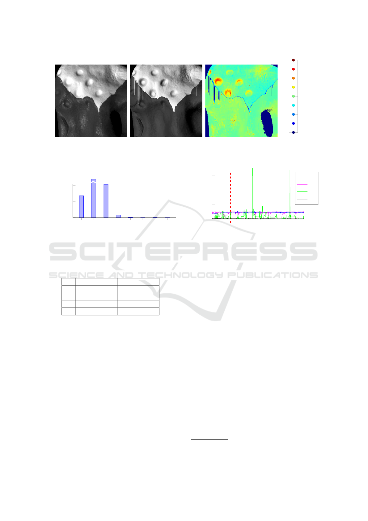
(a) (b) (c)
−0.2
−0.1
0
0.1
0.2
Figure 4: (a) One of the captured images, (b) reflectance map of segmented surface with computed parameters. Same scaling
of grey values in both images. (c) Absolute difference of intensity values.
1 2 3 4
5 6
7 8
0
500
1,000
682
13,178
1,037
79
7
3
12
2
model number m
# iterations
Figure 5: Histogram of visited models in model space.
Counting indicated that model 2 is the most likely.
Table 4: Maximum a-posteriori estimate of parameters and
1σ deviation for upper and lower region after burn-in phase
of 20%.
θ
i
upper Region lower Region
I
0
0.899 ± 0.029 0.241 ± 0.004
k
d
0.939 ± 0.098 0.968 ± 0.012
γ 0.338 ± 0.747 32.65 ± 4.068
σ
2
0.056 ± 0.007 0.016 ± 0.002
tribution. It is visible here as well that all parameters
except γ have converged fast to an almost stationary
value, whereas γ suffers from the small specular com-
ponent which makes its estimation difficult.
As already seen in Figure 4(b) the estimation of
the change points yields errors at the outer parts of the
object. The mode of the distribution of each change
point (blue line) and the 95% confidence level (ma-
genta dashed line) is shown in Figure 7(a). The yellow
box frames the region of high certainty that coincides
with the correct segmentation. The erroneous change
points yield a drastically increased uncertainty and as
such the algorithm itself is able to determine when to
trust a change point and when not.
A closer look at the estimated change points is
possible with Figure 7. The histogram of each change
point is given in Figure 7(b) and it is evident that the
correct segmentation has been part of the proposed
0 0.2 0.4
0.6
0.8 1 1.2
·10
4
0
2
4
6
iteration t
parameter value
I
0
k
d
γ
σ
2
Figure 6: Change of parameters of upper region for m = 2
(most likely model) throughout iterations. Most parame-
ters converge fast to an almost stationary value, γ shows a
higher uncertainty, the red dashed line indicates the end of
the assumed burn-in phase after 20% of the total iterations.
change point values and more often than other val-
ues as indicated by the color. Yet, many other change
points have been proposed and accepted such that the
resulting confidence level is low and the mode of the
distribution does not always coincide with the seg-
mentation ground truth.
A possible cause of the reduced quality of the seg-
mentation is the lack of data at the outer regions of
the object. Figure 8 shows the number of valid im-
ages per surface pixel. It is apparent that the outer ob-
ject surface yields less available information and thus
increases the difficulties of finding the correct change
points and BRDF parameters.
5 EVALUATION
To assess the prospects of the presented method,
we compare the results of the segmentation to com-
mon image segmentation procedures. We apply k-
means, e.g. (Seber, 1984; Spath, 1985), Gaussian
mixture model
2
(GMM) (McLachlan and Peel, 2000),
2
Matlab 2015a implementation of k-means and GMM.
Simultaneous Surface Segmentation and BRDF Estimation via Bayesian Methods
45
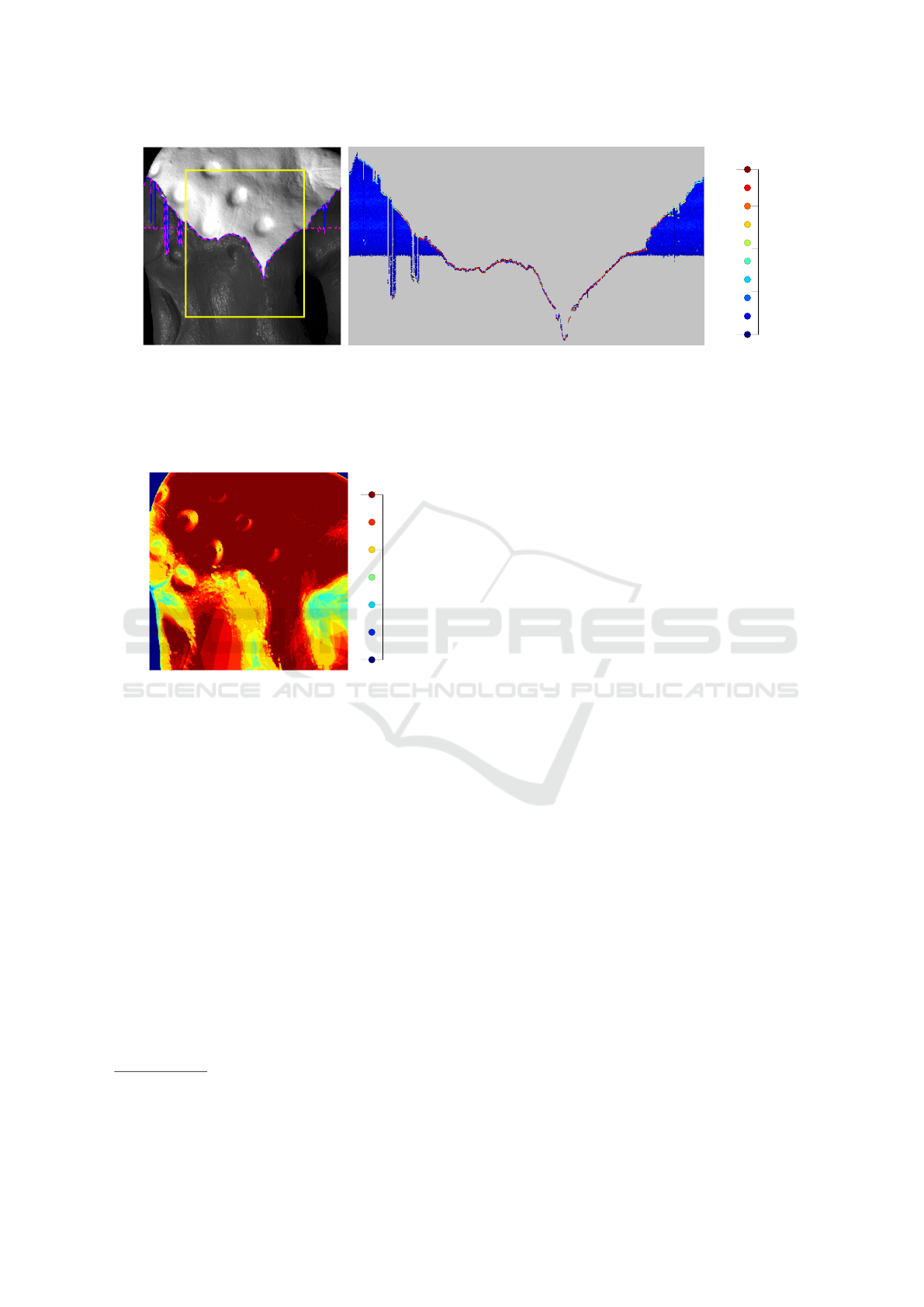
(a) (b)
0
20
40
60
Figure 7: (a) Position of change points (blue line) and 95%-confidence tube (magenta dashed line) showing the uncertainty.
The part inside the yellow box is segmented at high accuracy. The outer parts of the object show erroneous segmentation in
combination with an increased uncertainty. (b) 2D Histogram of change points after burn-in phase. Each column represents
the histogram of the respective change point in u direction, the color indicates the histogram counts per pixel. The image has
been zoomed to enlarge the area of interest and the square root has been applied to all counts to improve visibility.
0
6
12
18
Figure 8: Valid images per pixel available to the BRDF es-
timation. The outer region lacks data, which is caused by
shadowing or outlying illumination geometry and makes the
accurate BRDF estimation more difficult.
multichannel k-means (Pichler and Hosticka, 1995)
and normalized graph cuts
3
(NCuts) (Shi and Ma-
lik, 2000) segmentation procedures. The cluster al-
gorithms are applied to the synthetic data, since the
varying intensity and specular highlights are the more
challenging dataset to be accurately segmented.
Note that the comparison of these algorithms to
ours is questionable since the similarity criterion used
to dissect the surface is not the same in every pro-
cedure. Our methods operates on the average simi-
larity of measured grey values and a rendered image.
The segmentation procedures compared against our
method use grey values to dissect the image. In the
case of GMM we extended the input data with spatial
information about the pixel location. Furthermore,
NCuts can not handle multiple input images without
modification. However, to our knowledge there is no
3
We used the existing implementation provided at
http://www.cis.upenn.edu/ jshi/software/, last updated Jan-
uary 22, 2010.
method that yields a similar approach to image seg-
mentation as the one presented in this paper.
k-means. Multichannel image data can be ex-
ploited in a k-means clustering when treating each
of the P images as a separate feature of every pixel,
such that we get N · M samples (assuming I
NxM
) each
yielding P features. Since k-means requires that the
desired number of clusters is provided by the user,
we tried k ∈ [48]. The k-means segmentation of the
synthetic dataset is displayed in Figure 9. The seg-
mentation is erroneous for every considered number
of clusters. Since k-means operates on grey values,
the specular highlights of the surface determine the
dominant center of the clusters.
The multichannel k-means algorithm as described
by Pichler and Hosticka (1995) did not converge to a
solution on the given data.
Gaussian Mixture Model. Similar to the k-
means algorithm we supplied the multiple intensi-
ties per image pixel as features to the fitting of the
GMM. Moreover, we provided the spatial position of
the pixel as additional feature. The GMM is not able
to dissect the surface into the correct areas of different
reflectance properties as can be seen in Figure 10.
Normalized Cuts. Since the normalized cuts al-
gorithm is not designed to handle multispectral im-
age data only one image from the dataset (Fig 11(a))
is used to test the segmentation. To account for a
background-cluster the number of clusters k is in-
creased by one. Based on k ∈ {5, 6} the segmentation
appears reasonable, yet the borders are not perfectly
met. Increasing the number of clusters leads to false
segments instead of subdividing the correct segments
into smaller patches.
Note that the above mentioned segmentation pro-
cedures are superior to our method in computational
VISAPP 2016 - International Conference on Computer Vision Theory and Applications
46
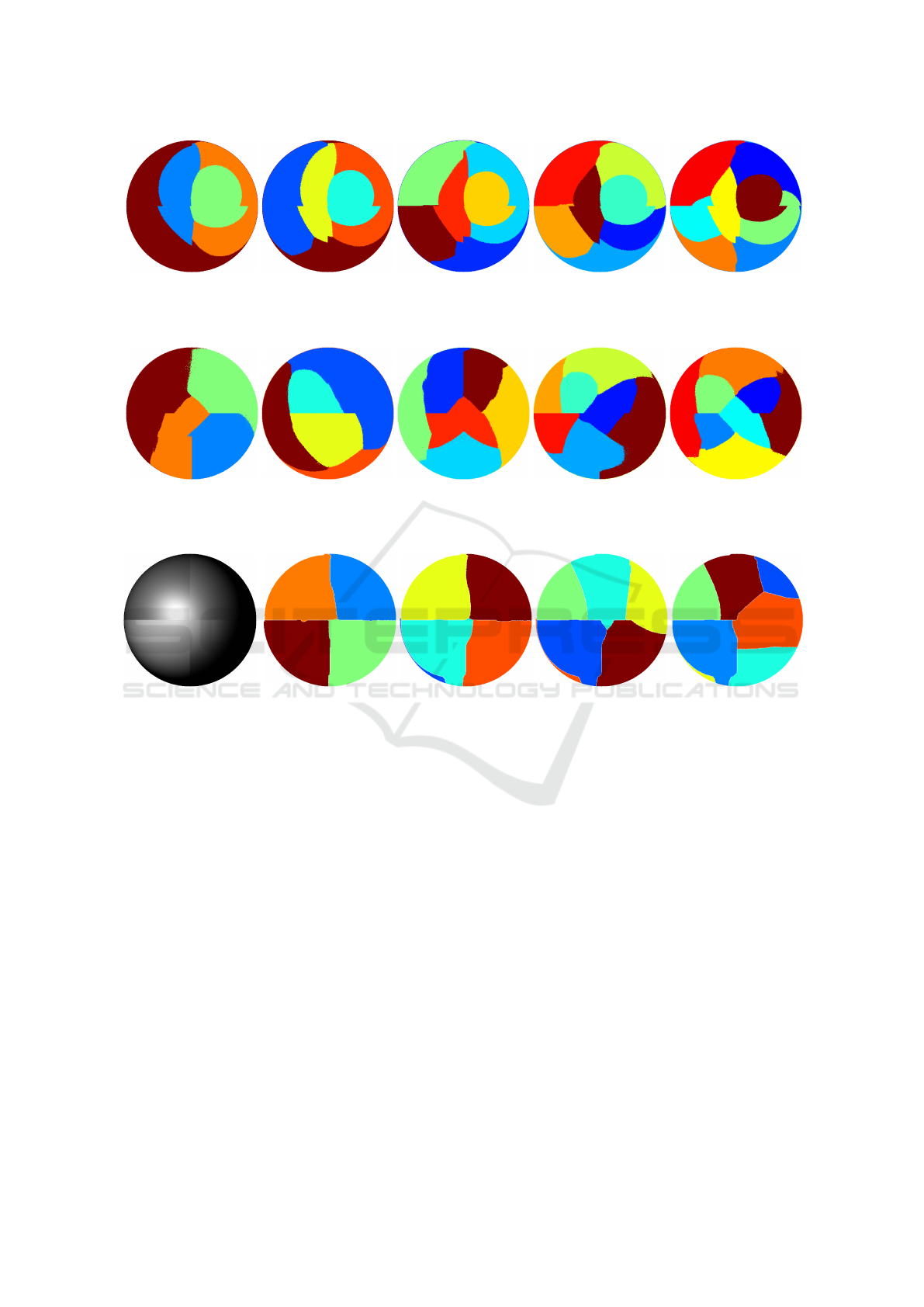
(a) k = 4 (b) k = 5 (c) k = 6 (d) k = 7 (e) k = 8
Figure 9: k-means segmentation of synthetic data, the colors code different surface segments. The segmentation fails for
every considered setting.
(a) k = 4 (b) k = 5 (c) k = 6 (d) k = 7 (e) k = 8
Figure 10: Gaussian mixture model segmentation of synthetic data, the colors code different surface segments. k is the number
of Gaussian distributions fit the data. The segmentation fails for every considered setting.
(a) (b) k = 5 (c) k = 6 (d) k = 7 (e) k = 8
Figure 11: a) Input image taken from the synthetic dataset. b)-e) Normalized cuts segmentation of synthetic data, the colors
code different surface segments. The number of clusters k is increased by one with regards to the actual number of surface
segments to account for a background cluster.
time. However, the general benefit of the Bayesian
approach is the inherent knowledge of the uncertainty
of the computed results. Furthermore, the reflectance
parameters of the segmented patches need to be com-
puted separately if e.g. used in surface reconstruction
applications such as shape from shading (Horn, 1986)
or photometric stereo (Woodham, 1980). Since the
surface segmentation in the presented algorithm is di-
rectly based on the reflectance estimation, the param-
eters of the surface segments including their uncer-
tainty are already known. Additionally, the methods
used for comparison require the number of desired
clusters as user input, which is not necessary in our
approach since it achieves unsupervised surface seg-
mentation.
6 CONCLUSIONS
In this paper we have shown that the segmentation
of an arbitrary surface is possible based on the maxi-
mum a-posteriori estimation of its reflectance param-
eters. The novelty of our procedure is the direct infer-
ence of patch borders and BRDF parameters from the
data and the computation based on Bayesian statis-
tics, which inherently allows us to deduce the accu-
racy of the computed results. The experimental eval-
uation has demonstrated that the amount of available
data has to be high enough to draw the correct con-
clusions from the input data.
In comparison to existing surface segmentation
procedures our method based on the surface re-
flectance properties achieves the best segmentation on
the synthetic dataset.
The proposal of new change points in the existing
Simultaneous Surface Segmentation and BRDF Estimation via Bayesian Methods
47

implementation is randomized and therefore favors
lines, which makes it difficult to segment circle-like
surface patches, since those have to be based on lines
that converge from opposing sides of the circle. Con-
sequently, a different concept of change point propo-
sition adapted from prior knowledge of the type of
surface segments would enhance the performance of
the procedure.
Furthermore, we would like to extend our method
to other BRDF (likelihood) functions which consider
Fresnel effects and shadowing/masking, e.g. (Cook
and Torrance, 1981), or introduce a more general co-
sine lobe model to cope for anisotropic reflection, e.g.
(Lafortune et al., 1997). Moreover, it is of great inter-
est to include the estimation of surface normals in the
likelihood, which would introduce two more param-
eters per pixel. This will probably increase the un-
certainty of the overall likelihood considerably, but at
the gain of freeing the procedure from the necessity
of any prior knowledge about the surface.
REFERENCES
Aittala, M., Weyrich, T., and Lehtinen, J. (2013). Practical
svbrdf capture in the frequency domain. ACM Trans-
actions on Graphics, 32.
Alldrin, N., Zickler, T., and Kriegman, D. (2008). Pho-
tometric stereo with non-parametric and spatially-
varying reflectance. Conference on Computer Vision
and Pattern Recognition.
Blinn, J. F. (1977). Models of light reflection for computer
synthesized pictures. Association for Computing Ma-
chinery’s Special Interest Group on Computer Graph-
ics and Interactive Techniques, 11(2):192–198.
Cook, R. L. and Torrance, K. E. (1981). A reflectance
model for computer graphics. Association for Com-
puting Machinery’s Special Interest Group on Com-
puter Graphics and Interactive Techniques, 15(3):307
– 316.
Giesen, F. (2009). Phong and blinn-
phong normalization factors. online
http://www.farbrausch.de/ fg/stuff/phong.pdf, 1:1–2.
Gilks, W., Richardson, S., and Spiegelhalter, D. (1996).
Markov Chain Monte Carlo in Practice. Chapman &
Hall.
Goldman, D. B., Curless, B., Hertzmann, A., and Seitz, S.
(2005). Shape and spatially-varying brdfs from photo-
metric stereo. International Conference on Computer
Vision, pages 341–348.
Green, P. J. (1995). Reversible jump markov chain monte
carlo computation and bayesian model determination.
Biometrika, 82:711–732.
Hastings, W. K. (1970). Monte carlo sampling methods us-
ing markov chains and their applications. Biometrika,
57:97–109.
Herbort, S. and W
¨
ohler, C. (2012). Self-consistent 3D sur-
face reconstruction and reflectance model estimation
of metallic surfaces. International Joint Conference
on Computer Vision, Imaging and Computer Graph-
ics Theory and Applications, pages 1–8.
Horn, B. K. P. (1986). Robot Vision. MIT Electrical Engi-
neering and Computer Science.
King, R., Morgan, B. J., Gimenez, O., and Brooks, S. P.
(2010). Bayesian Analysis for Population Ecology.
CRC Press.
Lafortune, E. P. F., Foo, S.-C., Torrance, K. E., and Green-
berg, D. P. (1997). Non-linear approximation of re-
flectance functions. Association for Computing Ma-
chinery’s Special Interest Group on Computer Graph-
ics and Interactive Techniques, pages 117–126.
Lambert, J.-H. (1760). Photometria, sive de mensura et
gradibus luminis, colorum et umbrae. Vidae Eber-
hardi Klett.
Laskey, K. and Myers, J. (2003). Population markov chain
monte carlo. Machine Learning, 50:175–196.
Lenoch, M., Herbort, S., Grumpe, A., and W
¨
ohler, C.
(2014). Linear unmixing in brdf reproduction and 3d
shape recovery. International Conference on Pattern
Recognition.
Lenoch, M., Herbort, S., and W
¨
ohler, C. (2012). Robust and
accurate light source calibration using a diffuse spher-
ical calibration object. Oldenburger 3D Tage, 11:212–
219.
Lensch, H. P. A., Kautz, J., Goesele, M., Heidrich, W., and
Seidel, H.-P. (2003). Image-based reconstruction of
spatial appearance and geometric detail. ACM Trans-
actions on Graphics, 22(2):234–257.
Louw, M. and Nicolls, F. (2010). Surface classification via
brdf parameters, using population monte carlo for mrf
parameter estimation. Proc. IASTED Int. Conf. Com-
puter Graphics and Imaging, 11:145–154.
Matusik, W., Pfister, H., Brand, M., and McMillan, L.
(2003). A data-driven reflectance model. ACM Trans-
actions on Graphics, 22(3):759–769.
McLachlan, G. and Peel, D. (2000). Finite Mixture Models.
John Wiley & Sons, Inc.
Metropolis, N., Rosenbluth, A., Rosenbluth, M., Teller, A.,
and Teller, E. (1953). Equation of state calculations
by fast computing machines. Journal of Chemical
Physics, 21:1087–1092.
Ntzoufras, I. (2011). Bayesian modeling using WinBUGS.
John Wiley & Sons.
Pichler, O. and Hosticka, A. T. B. J. (1995). A multichannel
algorithm for image segmentation with iterative feed-
back. In Image Processing and Its Application.
Seber, G. A. F. (1984). Multivariate Observations. John
Wiley & Sons, Inc.
Shi, J. and Malik, J. (2000). Normalized cuts and image
segmentation. Trans. Pattern Analysis and Machine
Intelligence, 8:888–905.
Spath, H. (1985). Cluster Dissection and Analysis: Theory,
FORTRAN Programs, Examples. Halsted Press.
Weyrich, T., Lawrence, J., Lensch, H., Rusinkiewicz, S.,
and Zickler, T. (2008). Principles of appearance ac-
quisition and representation. Association for Comput-
ing Machinery’s Special Interest Group on Computer
Graphics and Interactive Techniques, pages 1–70.
Woodham, R. J. (1980). Photometric method for determin-
ing surface orientation from multiple images. Optical
Engineering, 19(1):139–144.
VISAPP 2016 - International Conference on Computer Vision Theory and Applications
48
