
Robust Matching of Occupancy Maps for Odometry in
Autonomous Vehicles
Martin Dimitrievski, David Van Hamme, Peter Veelaert and Wilfried Philips
Vision Systems and Image Processing and Interpretation Research Groups, Ghent University,
Sint-Pietersnieuwstraat 41, Gent, Belgium
Keywords: Odometry, SLAM, Occupancy Map, Registration, 3DOF, LIDAR.
Abstract: In this paper we propose a novel real-time method for SLAM in autonomous vehicles. The environment is
mapped using a probabilistic occupancy map model and EGO motion is estimated within the same
environment by using a feedback loop. Thus, we simplify the pose estimation from 6 to 3 degrees of
freedom which greatly impacts the robustness and accuracy of the system. Input data is provided via a
rotating laser scanner as 3D measurements of the current environment which are projected on the ground
plane. The local ground plane is estimated in real-time from the actual point cloud data using a robust plane
fitting scheme based on the RANSAC principle. Then the computed occupancy map is registered against the
previous map using phase correlation in order to estimate the translation and rotation of the vehicle.
Experimental results demonstrate that the method produces high quality occupancy maps and the measured
translation and rotation errors of the trajectories are lower compared to other 6DOF methods. The entire
SLAM system runs on a mid-range GPU and keeps up with the data from the sensor which enables more
computational power for the other tasks of the autonomous vehicle.
1 INTRODUCTION
The technology advancement in sensors and
computer systems is enabling the proliferation of
Advanced Driver Assistance Systems (ADAS) into
the car market at an unprecedented pace. As of the
year 2015, systems such as adaptive cruise control,
automatic parking, automotive night vision, collision
avoidance, emergency braking, hill descent, lane
departure assistance, traffic sign recognition etc. can
be found as standard equipment even in the mid-
range vehicles on the market. Recent reports about
road safety indicate that driver error is the main
contributor to more than 90% of traffic accidents
(KPMG,2012), (Fagnant,2013). Even when the main
reason for a crash is due to malfunctions of the
vehicle or problems with the road or environment,
some additional human factors can often have
contributed to the crash and the severity of the
injuries. Leading companies involved in autonomous
vehicles believe that only completely self-driving
cars will fully address safety concerns.
Such intelligent vehicles make use of advanced
perception systems that could sense and interpret
surrounding environment based on various kinds of
sensors, such as: radar, lidar (laser rangefinder),
monocular / binocular / omnidirectional vision
systems, ultrasound, etc. Many of the following
tasks for the intelligent vehicle can be performed
within the same framework of sensory interpretation
(Leonard,2008), (Nguyen,2012). The initial tasks is
ego localization since the vehicle can’t drive safely
if it doesn’t know its location and orientation (i.e.
pose). The problem of pose estimation has been
exhaustively researched in various applications such
as stereo vision, structure from motion, mapping and
augmented reality, however one can conclude that
most of the proposed methods in the literature are
computationally expensive and do the estimation
off-line. The mainstream of approaches are based on
key feature detection in optical video frames, which
can be assessed by looking at the standard odometry
benchmark (Geiger, 2012 and 2013). Tracking and
registration of the detected features is often done
using the Iterative Closest Point (ICP) approach
(Pomerleau,2013). Pose estimation can also use the
data from inertial navigation sensors (INS), global
position system (GPS) or wheel rotation sensors, as
prior motion information in achieving real-time
computation speed (Scherer,2012). Kalman or
628
Dimitrievski, M., Hamme, D., Veelaert, P. and Philips, W.
Robust Matching of Occupancy Maps for Odometry in Autonomous Vehicles.
DOI: 10.5220/0005719006260633
In Proceedings of the 11th Joint Conference on Computer Vision, Imaging and Computer Graphics Theory and Applications (VISIGRAPP 2016) - Volume 3: VISAPP, pages 628-635
ISBN: 978-989-758-175-5
Copyright
c
2016 by SCITEPRESS – Science and Technology Publications, Lda. All rights reserved

particle filters are often used in order to reinforce the
measurements with the past data for more natural
estimation.
Figure 1: Small section of an occupancy grid map with
cell size 12.5x12.5cm.
When no additional data is available but the one
that comes from the stereo cameras and/or lidar,
many approaches have been proposed registering the
point clouds using a more suitable representation.
Notably, methods such as (Moosmann, 2011) use
projection of the point cloud onto a range image and
then use features extracted from these images to do
the matching between consecutive sweeps. On the
other hand, there are methods which try to extract
geometric primitives from within the point clouds,
such as planes and edges, and then use them for
matching and registration (Zhang,2014). These
approaches have their pitfalls in situations where the
environment does not contain simple planes and
edges (open roads, forests, parks). There are two
issues with these types of approaches: first, the high
computational cost for extracting the robust image
features and second, images in the visual spectrum
often fail to capture good information in adverse
weather conditions and during the night.
Therefore, we part with the standard 6DOF point
cloud registration paradigm and propose a novel
algorithm for simultaneously mapping the perceived
environment and performing the localization task
using the previous state of what has already been
mapped. We adopt the so called occupancy grid map
as a medium for all further operations of the
autonomous vehicle. In the literature, authors make
use of these logical representation, i.e. maps, which
explains the occupancy of the environment in a
probabilistic way, first proposed by (Moravec, 1985)
for use in sonar mapping.
Occupancy grid maps are spatial representations
of the external environment. The external world is
represented by a high resolution grid of variables
that model the occupancy of the space. Besides the
mapping the occupancy data can also be used for
various other key functions necessary for the mobile
vehicle navigation, such as positioning, path
planning, collision avoidance object detection and
prediction of the future state of the environment.
Older studies suggest that occupancy grid maps
are arguably the most successful environment
representation in mobile robotics to date
(Kortenkamp,1998). Moreover, in the domain of
autonomous vehicles, they are an optimal way of
recording a background model of the vast
environments, Fig.1. An efficient implementation of
these maps has been proposed by (Homm, 2010),
which will be explained in more detail in chapter 2.
We also make a simplification to the system
assuming that the world the vehicle is moving
through is completely flat and that it can be precisely
modelled via a two dimensional map. This way the
localization becomes a 3DOF registration problem
which can be solved robustly and more importantly,
with a tight real-time constraint. Our main sensor is
the Velodyne HDL-64E lidar which experiences the
same general motion as the vehicle: three degrees of
translational freedom and three degrees of rotation
relative to the environment. The pose estimation can
be seen as a closed feedback loop system that also
tries to produce a map of the environment using the
estimated pose information. A detailed analysis of
the classical pose estimation approach and our
simplified method follows in chapter 3.
The speed and accuracy of the proposed method
is experimentally tested in chapter 4 and we give our
concluding remarks in the discussion in chapter 5.
2 OCCUPANCY MAP
The proposed model of the environment estimates
the probability of occupancy for each world
coordinate using the inverse sensor logic. This
means that the sensor measurements are used to
reconstruct the most probable map using a Bayesian
reasoning. Occupancy maps can be a very elegant
solution to the problem of mapping when there is a
multitude of heterogeneous sensors on board the
vehicle. They are invariant to the category of the
scanned objects in the environment as long as they
are correctly transformed into probability of
occupancy. For example, one can incorporate
measurements from object detectors, ultrasound
Robust Matching of Occupancy Maps for Odometry in Autonomous Vehicles
629

objects, distance measures from lidar or stereo
cameras into one single occupancy map.
Let us define the occupancy map as a 2D grid
in the plane with grid elements
,
and a series
of
,...,
measurements obtained from the lidar. Each
sensor measurement
contains information about
the occupancy of several grid locations together with
the pose of the vehicle which might come from other
sensors. So, the problem of simultaneous building of
the map and localization of the vehicle can be
explained by finding the ego motion of the vehicle
using the previously built map and cumulatively
computing the probability of occupancy for each
grid element
,
given the new measurements in
.
We will first explain the update of the occupancy
map for a static vehicle, or a moving vehicle for
which we already solved the ego location. The
probability of occupancy for each grid element (cell)
can be estimated separately from the rest of the map
,
|
…
. (1)
Commonly the log-odds or log likelihood ratio
representation is used for computational reasons
since its update requires a simple addition operation,
,
,
|
…
1
,
|
…
,
(2)
where the posterior
,
can be reconstructed from
,
by
,
|
…
1
1
,
.
(3)
Since the error level of our sensor is lower than the
cell size, there is a high probability that most
measurements will fall within their respective grid
cells. Thus, we make an assumption that the
probability of occupancy of
,
is conditionally
independent of the rest of the map, even from its
neighbouring cells. We therefore can estimate the
posterior as
,
|
…
|
,
,
|
…
|
…
.
(4)
If we apply Bayes rule to the term
|
,
we
have the probability that the cell
,
is occupied:
,
|
…
,
|
,
|
…
,
|
…
.
(5)
The probability of the grid cell to be free
,
, can be
expressed with the same equation, and by noting that
,
,1
,
we can devise recursive
expression for the map update at time T given the
past map and the current measurements and pose:
,
,
|
1
,
|
1
,
,
,
,
(6)
where the initial map can be constructed from the
prior probabilities for occupancy for each grid cell:
,
,
1
,
.
(7)
This approach builds an incremental map of the
environment containing the log-odds for occupancy.
The first term of equation (6) explains the log-odds
of occupancy for a single cell given the
measurements in
, and the second term is the prior
log-odd of the cell. This relation is usually called an
inverse sensor model because it translates the sensor
measurements into their causes, i.e. the map. At any
given point one can recover the probability of
occupancy for the whole map using equation (3).
A more accurate approach to occupancy map
estimation is the forward sensor model which
computes the likelihood of the sensor measurements
in the space of all possible maps. This approach is an
optimization problem where we search an optimal
map which maximizes the probability of the given
measurements. However, the forward model
formulation prohibits a real-time implementation
since it requires every sensor measurement in order
to find the optimal map. We refer to (Thrun,2003)
for further information about the implementation of
the forward sensor model.
In the following chapter we will explain how the
pose estimation of the vehicle can be performed
using the currently unregistered occupancy map data
with relatively low computational complexity and
high level of accuracy.
3 POSE ESTIMATION
3.1 Classical 6DOF Approach
The pose of the sensor (lidar) corresponds to the
orientation and position of the vehicle, where in the
VISAPP 2016 - International Conference on Computer Vision Theory and Applications
630

first moment of time the pose is arbitrarily set at the
coordinate centre. As the vehicle is moving through
the world, it experiences rotational and translational
changes to its pose. The simplest forward motion on
a flat road produces a translation change in the axis
perpendicular to the vehicle motion, thus the vehicle
is moving with one degree of freedom. In the real
world though, the vehicle might be taking a turn in a
bend which has some incline (grade) and a slight
camber to the road surface. Furthermore, the vehicle
suspension will try to dampen the effects of the
forward and lateral acceleration and keep the vehicle
level to the ground. In these actual scenarios the
sensor attached to the vehicle is experiencing
changes within 6 degrees of freedom: motion in the
three spatial dimensions, and rotation around the
three axes, at the same time.
The problem of pose estimation then becomes
the standard problem encountered in structure from
motion applications where a 6DOF fundamental
matrix which explains the change of pose is being
estimated from the sensor data. Assuming that the
change in sensor data between two time intervals is
entirely due to motion through static environment,
then the 3D points measured in the present
are
related to the 3D points measured in the past
via the augmented matrix:
01
,
(8)
where the points are expressed in homogeneous
coordinates,
represents the 3x3 rotation matrix
and
represents a 3x1 translation vector. The pose
can thus be estimated by finding the optimal
transformation matrix which minimizes the distance
between the two sets of 3D points after
transformation. Although elegant, the solution of the
ego motion is a typical non-linear least squares
problem which is highly sensitive to noise. Several
existing approaches can minimize or remove noisy
data from the system at different points. A widely
used technique is the Iterative Closest Point
algorithm (Chen,1991) which is effectively applied
in matching point cloud data by iteratively searching
for the nearest neighbours for each point. Another
popular method is the Random Sample Consensus
which is designed to cope with large percentages of
outliers in the data (Fischler, 1981) and can be
applied to iteratively estimate the rotation and
translation by using a subset of 3D points which
produce the maximum number of inliers.
Directly matching the point clouds generated by the
lidar sensor cannot produce accurate results because
of the non-uniform sampling technique of the
rotating head, so most authors are adapting their
methods to search for suitable geometric primitives
within the point clouds and use them as features for
further matching. Other types of approaches try to
estimate the geometric primitives by projecting the
point clouds onto a 360 degree panoramic image and
use it to find robust features for matching. However,
the autonomous vehicle does not always encounter
regularly shaped manmade objects and most of the
time when driving on open roads the surrounding
objects are of natural origin. This relative scarcity of
geometric primitives in the point-cloud data can
render most of the geometrically based matching
algorithms ineffective since they discard a lot of
otherwise useful information.
3.2 Proposed Method
We are guided by the idea that no information from
the sensors should be discarded and as such, the
whole lidar point cloud should be used as a single
feature for pose estimation. Since the objective in
our project is SLAM with additional object detection
within the built environment model, we adopt the
occupancy map as a feature and use what
information is available from the past measurements
for registration. Among other benefits, this also
makes the system design feasible for real-time
application. From the experimental runs of the
vehicle and the acquired point clouds we can
observe that the car is moving in a relatively flat
environment (low absolute road grade compared to
the range of the sensor). The change in elevation
between two consecutive laser scans falls below the
noise threshold of the sensor. This motivates us to
assume that the occupancy of the environment can
be modelled using a flat two dimensional map, an
important simplification to the pose estimation
problem which brings higher accuracy and fast
execution times.
The algorithm starts by finding the ground plane,
i.e. the 3D plane on which most of the road surface
is laid on. The flat world assumption dictates that
any difference of the estimated ground plane and the
world plane (z=0) is due to sensor rotation. This can
happen because of the dynamics of the vehicles’
suspension during linear or lateral accelerations and
most notably while passing speed bumps or
potholes.
We use an iterative plane fitting algorithm on the
raw point cloud data to select the three points that
best explain the road surface. It is based on the
paradigm of RANSAC in a way that in each iteration
a random subsample of points is used to generate a
Robust Matching of Occupancy Maps for Odometry in Autonomous Vehicles
631
plane equation for which the average distance of all
other points is computed and the subset with the
lowest average distance (highest number of inliers)
is selected. From the list of inliers
of this optimal
subset, a new plane is fitted in a least squares sense.
The point cloud is then “rectified” relative to this
ground plane by applying the inverse rotation
relative to the estimated ground normal.
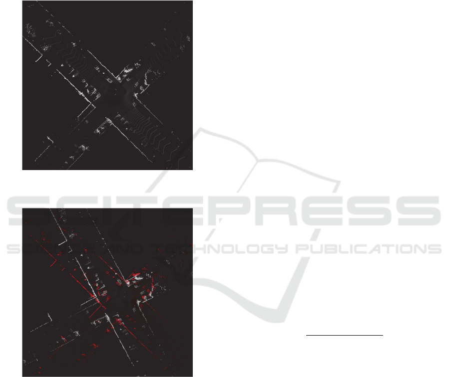
Figure 2: Example of the initial occupancy map, the black
background is assumed to be free (p=0).
Figure 3: Comparison of two occupancy maps with
temporal difference of 500ms (red colour now codes the
past information, same as Fig.2).
The next step is the projection of the rectified
point cloud on the world plane to produce the initial
occupancy map. We accumulate the height of each
3D point into the respective occupancy grid cell and
produce a probability of occupancy based on the
average height of points over that location. Points
with height greater than 3m are assumed to be have
a probability of 1 and points in between are scaled
respectively, Fig.2. Thus, we obtain an orthographic
projection of the environment in a form of a top
view. Vehicle rotation will produce rotation of the
features on the map, and vehicle translation will shift
the rows and columns of the map. One can clearly
see the actual change in rotation and position of
features on Fig.3. where the initial occupancy map is
compared with the occupancy map produced after
500ms of driving.
We will focus on this domain of imagery to
estimate the current pose of the vehicle using
standard image registration techniques. The aim is to
estimate the rotation and translation change between
two occupancy maps built from the sensor data of
two consecutive positions. We adopt the widely used
technique of Phase-Only Correlation (POC)
(Nagashima,2007) which naturally decouples the
rotation estimation from the translation estimation in
a two step approach. The input occupancy maps are
transformed using the 2D DFT
,
,
,
,
1
,
1
,
,
(9)
where their respective amplitude spectra
,
and
,
1
are shift-invariant and
thus can be used for rotation estimation. In order to
directly estimate the rotation change we further take
the log of each spectra and transform it in polar
coordinates (
,
), thus the rotation estimation boils
down to shift estimation. This is easily computed
using the 2D convolution of these two images using
the normalized cross-power spectrum
,
,
,
,
,
(10)
where
,
is the complex conjugate of the
polar log spectrum of the occupancy map at time T-
1.The phase-only correlation is defined by the
inverse discreet Fourier transform of (10). If the two
input images are the same, then the POC function is
the Kronecker delta function and the more the two
images differ the more the peak height reduces and
there is an apparent shift in the actual position of the
peak. Peak height in the POCC function is a good
measure of the similarity of the two images and the
position of the peak is proportional to the angle of
rotation in the pose of the vehicle. In our
experiments we estimate the peak of the POC
VISAPP 2016 - International Conference on Computer Vision Theory and Applications
632
function by parabolic fitting and thus estimate the
rotation of the vehicle with sub “pixel” accuracy.
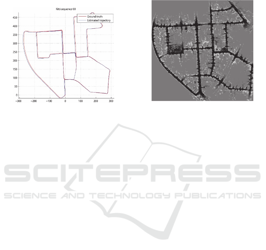
Figure 4: Estimated trajectory vs. trajectory recorded using
GPS/IMU for KITTI sequence 00, scale in [m].
Once the rotation has been estimated, the old
occupancy map is rotated to match the current. The
remaining difference, the shift of the two maps, is
due to the forward translation of the vehicle which is
again estimated similarly using the POC function
from equation (10). It is important to note that we
use a weighting function in a form of a low pass
filter for the Fourier coefficients in order to reduce
the effect of lidar noise introduced in the measured
points and the presence of moving objects in the
scene.
The output of the spectral matching is the yaw
angle delta of the vehicle between two consecutive
sensor measurements and the magnitude of the
translation vector in 2D space. In order to predict the
actual X,Y position of the vehicle and its exact
trajectory we multiply the translation magnitude by
the cosine and sine of the yaw delta and accumulate
the results over time
∗
∗sin
,
(11)
where Trans is the estimated translation change
between two consecutive scans.
This information is fed back to the mapping
equation (6) as part of the measurement
in order
to correctly project the lidar points on the global
occupancy map of the environment. An example of a
computed trajectory after several minutes of driving
a loop through a public road can be seen on Fig.4,
and the resulting occupancy map that has been
generated on fig.5.
Figure 5: Estimated occupancy map for KITTI 00.
4 EXPERIMENTS AND RESULTS
For validation we use the raw data streams provided
by the lidar recordings from the KITTI dataset, and
perform our mapping and registration analysis. We
chose this particular dataset as it is currently the
most comprehensive study about autonomous
vehicles driving through public roads. The
experimental dataset contains 21 recordings from
driving the vehicle through urban, rural and highway
roads. These recordings were made with the rotating
lidar and two stereo camera pairs. We only used the
data from the lidar which is rotating at 10Hz
providing an aggregated point cloud every 100ms.
Each point of the point cloud is defined with X,Y,Z
Cartesian coordinates and a reflectance index.
Additionally, a 6DOF pose matrix is given for each
time instance. We will compare our trajectories to
the GPS poses in order to measure the accuracy of
the pose estimation, but since there is currently no
ground truth data available for evaluating the
occupancy mapping system, the map accuracy will
only be measured qualitatively.
Our estimated odometry poses contain
information for 3DOF changes of the vehicle. We
use the method for evaluation suggested by the
authors of the KITTI dataset in order to compare the
accuracy of the estimated trajectories, i.e. we
compute the average rotation and translation errors
for every segment of length 100,200... 800m. For the
sequences which have GPS ground truth data
available, {0..10}, we report an average 3DOF
rotation error of 0.00380 deg/m and average 3DOF
translation error of 0.2904% measured as an average
Robust Matching of Occupancy Maps for Odometry in Autonomous Vehicles
633

differences between the starting and ending poses
for each sub-segment of length 100m to 800m using
the distance metrics as follows:
,
min2
|
|
,
|
|
∆
,
,
∈
100,200,…,800
1
∆
,
,∆
,
,
(12)
where is the smallest distance between two angles,
is the start of each sub-trajectory and is the total
number of sub-trajectories evaluated. For measuring
the error in the Yaw angle, we extract the Yaw from
each pose matrix of the ground truth and input it into
equation (12). The 3DOF translation error is simply
the average difference of the
norms of each start
and end position for the ground truth and estimated
sub-trajectories.
We also uploaded our results on the test server
provided by the authors of the dataset to evaluate
how this approach compares against other 6DOF
algorithms. The 6DOF pose errors measures the
angular and translational difference of the start and
end pose matrix
in 3D :
,
(13)
Our 6DOF pose matrices are constructed by
transforming the three Euler angles and the 2D
translation vector into a 3x4 matrix using the
estimated Yaw angle and zeros for the roll and pitch,
also, we use zero value for the height. Hence is the
expected drop in accuracy measured using the test
server of the KITTI dataset.
Table 1 holds a summary for the accuracy of the
results obtained with our algorithm compared to the
other methods. The entire table and other
information about the methods can be found at
(KITTI, 2015), however, in this extract we included
the top performing methods by means of translation
error and one of the rare methods based solely on
lidar point cloud data “
pcl-ndt-gicp”. As expected,
our approach has mediocre accuracy when tested on
the full 6DOF benchmark with the missing non
estimated data, scoring 1.89% average translation
error and 0.0083 deg/m average rotation error.
However, the 3DOF poses that we estimate score the
highest accuracy on the list for translation error.
We further investigated the robustness of our
method by adding two types of noise to the point
clouds. In the first experiment, the data is polluted
with additive white Gaussain noise in all of the three
spatial dimensions. The standard deviation of the
distribution is increased within reasonable ranges [5-
100cm] simulating point-clouds from a low-end
laser scanner. In the second experiment we have
kept the original points from the lidar intact only we
adding new points which simulate erroneous data i.e.
outliers which might be produced from other
sensors. The rate of outlier pollution, again, was
increased within reasonable ranges [2.5-90%].The
resulting 3DOF rotation and translation errors for the
KITTI dataset are measured as previously described.
We observed that the proposed method is able to
cope well with large amounts of both additive noise
and the presence of outliers. The translation error
seems to sharply increase once an additive error of
more than 70cm is added to the lidar data or once
there are more than 60% outlier points. This
robustness is due to the nature of the spectral
matching pose estimation.
Table 1: Average rotation and translation errors in 6DOF
for the test sequences of the KITTI dataset.
Method Terr. Rerr. Exec. time Environ.
V-LOAM 0.75% 0.0018 0.3s 4xCPU
LOAM 0.88% 0.0022 1s 2xCPU
SOFT 1.03% 0.0029 0.1s 2xCPU
Cv4xv1-sc 1.09% 0.0029 0.145s GPU
...
PROPOSED
3DOF
0.29% 0.0038 0.05s GPU
PROPOSED
6DOF
1.89% 0.0083 0.05s GPU
pcl-ndt-gicp 2.02 0.008 2s 10xCPU
Our GPU implementation has an execution time
which can keep up with the lidar data. The algorithm
is running at around 20fps on a mid-range graphics
card. The registration of the occupancy maps
consumes around 30-40ms and the rest is spent on
the RANSAC and fitting for the ground plane
estimation (10-20ms).
5 CONCLUSION
We proposed a feedback loop approach for SLAM
by using the probabilistic occupancy map model. By
simplifying the pose estimation problem in the
3DOF domain of the occupancy map we have
managed to achieve high accuracies for both
translation and rotation estimation. The resulting
trajectories correspond very well to the orthographic
projections of the path the vehicle is taking and the
built maps accurately reflect the occupancy
situation. By avoiding the time consuming and often
unreliable stereo video feature matching approach
we managed to localize the vehicle using only the
VISAPP 2016 - International Conference on Computer Vision Theory and Applications
634

laser scanner point clouds in their entirety as a single
feature.
However, the laser scanner produces point
clouds that are oftentimes are subjected to clearly
visible rolling shutter effect. Few authors in the past
have pointed out this problem when trying to use the
raw point clouds as input for odometry, and different
de-warping techniques have been used in order to
produce an accurate image of the environment. This
is done relying on additional sensors for motion
prior which in our project were not fully available.
We demonstrated that by using the warped point
clouds provided by the KITTI dataset the occupancy
map registration algorithm can produce accurate
enough results for the purpose of mapping and later
object detection of the autonomous vehicle. We
point reader to observe a detailed crop from one of
the built occupancy maps on Fig.1 and also to check
the integrity of the built map shown on Fig.5.
The main drawback of our method is an actual
result of the simplification of the problem and can
happen when the vehicle crosses its own path over a
bridge. The method is currently unable to put the
height difference into the occupancy map.
ACKNOWLEDGEMENTS
The work was financially supported by IWT through
the Flanders Make ICON project 140647
“Environmental Modelling for automated Driving
and Active Safety (EMDAS)”.
REFERENCES
KPMG (2012), “Self-Driving Cars: The Next Revolution”,
KPMG and the Center for Automotive Research; at
www.kpmg.com/Ca/en/IssuesAndInsights/ArticlesPub
lications/Documents/self-driving-cars-next-revolution.
pdf.
Daniel J. Fagnant and Kara M. Kockelman (2013),
“Preparing a Nation for Autonomous Vehicles:
Opportunities, Barriers and Policy
Recommendations”, Eno Foundation; at
www.enotrans.org/wpcontent/uploads/wpsc/download
ables/AV-paper.pdf.
John Leonard. “A perception-driven autonomous urban
vehicle”. Journal of Field Robotics, vol. 25, pages
727-774, October 2008.
Thien-Nghia Nguyen, Bernd Michaelis and Al-Hamadi.
“Stereo Camera Based Urban Environment Perception
Using Occupancy Grid and Object Tracking”. IEEE
Trans. on Intelligent Transportation Systems, vol. 13,
pages 154-165, March 2012.
A. Geiger, P. Lenz, and R. Urtasun, “Are we ready for
autonomous driving? The kitti vision benchmark
suite,” in IEEE Conf. on Computer Vision and Pattern
Recognition (CVPR), 2012, pp. 3354–3361.
A. Geiger, P. Lenz, C. Stiller, and R. Urtasun, “Vision
meets robotics: The KITTI dataset,” Int. Journal of
Robotics Research, no. 32, pp. 1229–1235, 2013.
F. Pomerleau, F. Colas, R. Siegwart, and S. Magnenat,
“Comparing ICP variants on real-world data sets,”
Autonomous Robots, vol. 34, no. 3, pp. 133–148,
2013.
S. Scherer, J. Rehder, S. Achar, H. Cover, A. Chambers,
S. Nuske, and S. Singh, “River mapping from a flying
robot: state estimation, riverdetection, and obstacle
mapping,” Autonomous Robots, vol. 32, no. 5, pp. 1 –
26, May 2012.
F. Moosmann and C. Stiller, “Velodyne SLAM,” in IEEE
Intelligent Vehicles Symp. (IV), Baden-Baden,
Germany, June 2011.
J. Zhang and S. Singh, “LOAM: Lidar Odometry and
Mapping in Real-time”. Robotics: Science and
Systems Conf. 2014.
H. Moravec and A. Elfes. “High resolution maps from
wide angle sonar”. In In Proc. of the IEEE Int. Conf.
on Robotics & Automation (ICRA). volume 2, pages
116121, Mar. 1985.
D. Kortenkamp, R.P. Bonasso, and R. Murphy, editors.
“AI-based Mobile Robots: Case studies of successful
robot systems”, Cambridge, MA, 1998. MIT Press.
Homm, F. BMW Group, Res. & Technol., Munich,
Germany, Kaempchen, N. ; Ota, J. ; Burschka, D.
“Efficient Occupancy Grid Computation on the GPU
with Lidar and Radar for Road Boundary Detection”,
2010 IEEE Intelligent Vehicles Symp. University of
California, San Diego, CA, USA June 21-24, 2010
Sebastian Thrun, “Learning Occupancy Grid Maps with
Forward Sensor Models”, Journal Autonomous
Robots, Vol. 15 Issue 2, Sept. 2003 Pages 111 – 127
Y. Chen and G. Medioni, “Object modeling by registration
of multiple range images,” in IEEE Int. Conf. on
Robotics and Automation, 9-11 April 1991, pp. 2724 –
2729.
Martin A. Fischler and Robert C. Bolles. “Random sample
consensus: a paradigm for model tting with
applications to image analysis and automated
cartography”. Communications of the ACM, vol. 24,
pages 381-395, 1981.
Sei Nagashima, Koichi Ito, Takafumi Aoki, Hideaki Ishii,
Koji Kobayashi, “A High-Accuracy Rotation
Estimation Algorithm Based on 1D Phase-Only
Correlation”, ICIAR'07 Proceedings of the 4th
international conference on Image Analysis and
Recognition Pages 210-221
KITTI odometry results, available on:
http://www.cvlibs.net/datasets/kitti/eval_odometry.php
Robust Matching of Occupancy Maps for Odometry in Autonomous Vehicles
635
