
Direct Stereo Visual Odometry based on Lines
Thomas Holzmann, Friedrich Fraundorfer and Horst Bischof
Institute for Computer Graphics and Vision, Graz University of Technology, Graz, Austria
Keywords:
Visual Odometry, Pose Estimation, Simultaneous Localisation and Mapping.
Abstract:
We propose a novel stereo visual odometry approach, which is especially suited for poorly textured environ-
ments. We introduce a novel, fast line segment detector and matcher, which detects vertical lines supported
by an IMU. The patches around lines are then used to directly estimate the pose of consecutive cameras
by minimizing the photometric error. Our algorithm outperforms state-of-the-art approaches in challenging
environments. Our implementation runs in real-time and is therefore well suited for various robotics and
augmented reality applications.
1 INTRODUCTION
In the last years, Simultaneous Localization and Map-
ping (SLAM) and Visual Odometry (VO) became an
increasingly popular field of research. In comparison
to Structure from Motion (SfM), which is not con-
strained to run in realtime, SLAM and VO methods
should be able to run in realtime even on lightweight
mobile computing solutions.
Visual localization and mapping approaches are
often used for small robotics devices (e.g. Micro
Aerial Vehicles (MAVs)), where it is not possible to
use heavier and more energy-consuming sensors like
laser scanners. However, most of these devices are
equipped with an Inertial Measurement Unit (IMU),
which can be used in conjunction with vision meth-
ods to improve the results.
There exist widely used monocular SLAM/VO
methods, which just use one camera as the only in-
formation source and therefore can be used on many
different mobile devices. In contrast to monocular
approaches, stereo VO methods using a stereo setup
with a fixed baseline have some benefits, especially
when used for Robotics: (1) Monocular approaches
cannot correctly determine the metric scale of a scene,
while stereo approaches do have a correct scale as
the baseline of the camera setup is fixed. Addition-
ally, monocular approaches also have a drift in scale.
(2) Monocular approaches do have problems with
pure rotations as no new 3D scene information can
be computed from images without translational move-
ment. Contrary, stereo approaches do not have this
problems, as a stereo rig already contains translation-
ally moved cameras to triangulate scene information
regardless of the motion of the cameras.
Based on the observation that man-made scenes
usually contain strong line structures, like, e.g, doors
or windows on white walls, we especially want to
use these structures in our approach. Current feature-
point based methods (e.g. (Geiger et al., 2011)) have
problems in these scenes, as the lack of texture leads
to a low number of detected feature points. Direct
pose estimation methods (e.g. (Engel et al., 2014))
directly use the image information to align consecu-
tive frames and do not use explicitly detected feature
point correspondences to estimate the camera pose.
Therefore, direct methods perform better in poorly
textured environments, as they use more image infor-
mation and do not rely on detected feature points in
the scene.
In this paper, we present a pose estimation
method specifically targeted at poorly textured indoor
scenes where other methods deliver poor results. We
estimate the pose of a camera by minimizing the pho-
tometric error of patches around lines. We introduce
a fast line detector which detects vertical lines aided
by an inertial measurement unit (IMU). In case too
few lines could be detected, we additionally detect
point features and use patches around the detected
points for direct pose estimation. In our experiments
we show that our method outperforms state-of-the-art
monocular and stereo approaches in poorly textured
indoor scenes and delivers comparable results on
well textured outdoor scenes.
476
Holzmann, T., Fraundorfer, F. and Bischof, H.
Direct Stereo Visual Odometry based on Lines.
DOI: 10.5220/0005715604740485
In Proceedings of the 11th Joint Conference on Computer Vision, Imaging and Computer Graphics Theory and Applications (VISIGRAPP 2016) - Volume 3: VISAPP, pages 476-487
ISBN: 978-989-758-175-5
Copyright
c
2016 by SCITEPRESS – Science and Technology Publications, Lda. All rights reserved

To summarize, our main contributions are:
• A direct stereo VO method using lines running in
real-time.
• A novel efficient line detection algorithm aided by
an IMU, that detects vertical lines.
• A fast line matching technique using a lightweight
line descriptor.
2 RELATED WORK
A widely used approach to estimate the pose of a
camera using the image data only is to use feature
points in images. Feature points are detected and
matched between subsequent images and used to es-
timate the pose of the camera. A popular monocu-
lar point-based SLAM-approach is PTAM (Klein and
Murray, 2007). It runs in real-time and is specifically
designed to track a hand-held camera in a small aug-
mented reality workspace. However, there also exist
adoptions tailored at large-scale environments ((Mei
et al., 2010), (Weiss et al., 2013)). As it needs to de-
tect and match feature points, the environment has to
contain sufficient texture suited for the feature point
detection algorithm. Additionally, as it is a monocular
approach, it has difficulties in handling pure rotations
and cannot estimate a correct scale of the scene. A
feature-based approach, which uses a stereo camera
as input and therefore does not have this problems is
Libviso (Geiger et al., 2011). However, as it also uses
explicitly detected feature points, the texture needs to
be adequate for the detection algorithm. Additionally,
as it is not a SLAM method like PTAM but just a VO
method, it does not compute a global map of the en-
vironment but just computes the relative pose from
frame to frame.
Instead of using points, also lines can be detected
and matched in order to compute the pose of a cam-
era. In (Elqursh and Elgammal, 2011), Elqursh et al.
propose to estimate the relative pose of two cameras
by using three lines having a special primitive config-
uration. This has the advantage that no texture at all
needs to be present, but just a special line configura-
tion has to exist. However, as explicit line detection
is relatively slow, this approach cannot be used on a
low-end onboard computer.
Recently, direct pose estimation algorithms be-
came popular. In comparison to feature point-based
approaches, direct approaches do not explicitly detect
and match features and compute the pose using the
feature matches, but compute the new pose by mini-
mizing the photometric error over the whole or over
big parts of the image. For example, DTAM (New-
combe et al., 2011) tracks the pose of a monocular
camera given a dense model of the scene, by minimiz-
ing the photometric error of the current image accord-
ing to the whole model. As this is a computational
expensive task, a high-performance GPU is necessary
to compute the pose in real-time. Similarly, LSD-
SLAM (Engel et al., 2014) computes the pose by min-
imizing the photometric error. However, to reduce
computational cost, it just uses areas in the image
where the image gradient is sufficiently high. There-
fore, it runs in real-time even on hand-held devices
like smartphones. Also an extension of LSD-SLAM
to a stereo setup has been proposed recently (Engel
et al., 2015). In (Forster et al., 2014), an approach
is proposed which uses both explicit feature point
matching and direct alignment and is therefore called
semi-direct visual odometry (SVO). It detects feature
points at keyframes and computes the poses of im-
ages between keyframes by minimizing the photomet-
ric error of patches around the feature points. It runs
very fast even on onboard computers and is specif-
ically designed for a downwards looking camera of
a micro aerial vehicle. In summary, direct methods
perform direct image alignment to estimate the pose
of a new frame with respect to previously computed
3D information by optimizing the pose parameters di-
rectly and by minimizing a photometric error. This is
in contrast to feature-based methods, where features
are detected and matched to compute the fundamen-
tal matrix, and optimization is just optionally used to
refine the computed poses by using the reprojection
error.
Our method is a direct method, but utilizes a stereo
camera rig instead of a monocular camera. In contrast
to all previous related work, we detect lines and esti-
mate the pose by minimizing the photometric error
of patches around the lines. Using our line detector,
it is possible to detect lines very fast in constrained
images. As in man-made environments most of the
structure consists of lines, using patches around lines
is usually sufficient to directly align consecutive im-
ages.
3 DIRECT VISUAL ODOMETRY
BASED ON VERTICAL LINES
In our approach, we explicitly use the structures
contained in man-made environments to introduce a
novel visual odometry approach.
Instead of directly aligning the whole image or
explicitly detecting and matching feature points, we
estimate the camera pose by aligning patches just
around detected lines by minimizing the photometric
error. In case no lines can be detected, feature points
Direct Stereo Visual Odometry based on Lines
477
Input:
Stereo Images
IMU Measurements
Triangulate New
3D Information
Gravity Alignment
Direct
Pose Estimation
Propagate 3D Map
To Current View
Feature Detection
(Lines / Points)
Keyframe
Output:
Camera Pose
Local
Map
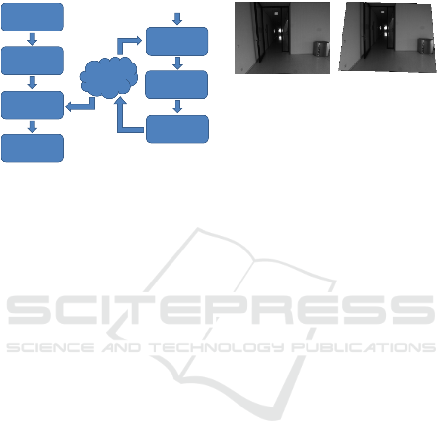
Figure 1: Overview of the processing pipeline. Our algo-
rithm directly estimates the pose of the camera by minimiz-
ing the photometric error of patches around vertical lines.
For every keyframe, the 3D information from the previous
keyframe gets projected into the current one, new lines and
optionally points get detected and new 3D information is
triangulated within the stereo setup.
are detected and patches around the points are used
for image alignment.
3.1 System Overview
Our approach is a keyframe-based stereo approach,
which takes rectified stereo images and optionally
synchronized IMU values as input. As preprocess-
ing, we align the images according to the gravity di-
rection using the IMU measurements. Without IMU
measurements, our approach also works on images
acquired with roughly gravity aligned cameras.
For every keyframe, we detect and match lines us-
ing gravity-aligned stereo images. If not enough lines
can be matched, we additionally detect and match
point features. We triangulate this information to get
a mapping of the visible information in 3D. A new
keyframe is selected when the photometric proper-
ties of the images changed too much or the movement
w.r.t the last keyframe is too big.
For every image, the pose gets estimated by direct
image alignment: We project all triangulated informa-
tion of the previous keyframe into the current image
and estimate the pose by minimizing the photometric
error of patches around the lines and points.
Additionally, for every consecutive keyframe, we
project lines and points from the previous one into the
current one to reuse already computed 3D information
if the same lines or points are detected.
In Fig. 1, one can see a schematic overview of our
processing pipeline.
Figure 2: Image alignment according to the gravity direc-
tion. Left: An unaligned image from a forwards looking
camera Right: Image aligned using the IMU. As one can
see, having an image aligned according to the gravity direc-
tion, straight, vertical lines in the 3D scene are mapped to
straight, vertical lines in the image.
3.2 Fast Line Detection and Matching
Areas around lines contain high gradient values which
is an important property for direct image alignment.
Therefore, we introduce a fast line detection and
matching method, where the area around lines is used
for direct image alignment afterwards. We compute
the depth of the lines by computing the disparity of
the lines using the stereo image pair.
3.2.1 Line Detection
Usually, line detection (like, e.g. (Grompone et al.,
2010)) is too slow for real-time applications (Hofer
et al., 2014). To make the problem feasible, we focus
on the detection of vertical lines, which can be done
much faster. Man-made environments usually contain
many vertical lines. Especially indoors, where the
texture available very often mainly consists of lines,
it is crucial for a visual odometry approach to use
also this information. We introduce a detection al-
gorithm aided by IMU information to make this chal-
lenging line detection step feasible: Having cameras
with arbitrary poses and synchronized IMU informa-
tion as input, the images can be aligned with the grav-
ity direction using the simultaneously acquired IMU
data (see Fig. 2). As the angular accuracy of IMUs is
quite high (e.g., evaluation of the IMU of the Pixhawk
autopilot (Cortinovis, 2010)) and most of the mobile
computing devices already contain built-in IMUs, this
preprocessing step can be done with many available
mobile computing devices.
Even if the alignment is not completely perfect,
it does not influence the pose estimation step, as the
lines are not directly used for pose estimation but in-
stead the patches around them. Errors in the align-
ment just result in a poorer line detection performance
which can lead to shorter detected lines.
Assuming gravity aligned images as input, the
task of detecting vertical lines gets easier as real-
world vertical lines are now projected to vertical lines
VISAPP 2016 - International Conference on Computer Vision Theory and Applications
478

Figure 3: Vertical lines detected with our line detection al-
gorithm. One can see that the lines are not detected over
the whole length all the time. This is due to slight gravity
misalignment of the images or due to changing light condi-
tions.
in the image. Using this assumption, our algorithm
first computes the image gradient in horizontal direc-
tion by convolving the image with the Sobel operator.
Next, for every column of the image, a histogram of
the gradient values is created. When a histogram bin
associated with sufficiently high gradient values con-
tains enough elements, a line is detected in this col-
umn.
As the lines are detected with pixel accuracy and,
therefore, the number of lines is limited by the num-
ber of columns, we have a small and limited number
of lines which increases the speed of the following
line matching step.
After the detection of lines, we apply a simple
non-maxima suppression: Lines get accepted, if their
corresponding gradient histogram bin contains more
elements than every gradient histogram bin corre-
sponding to nearby lines.
Finally, the start and end point of the line is de-
tected. In the gradient image, we search along the
associated column for the first pixel belonging to the
same bin as the corresponding line bin. This defines
the start point of the line. Next, we search for a pixel
belonging to a different bin. This defines the end point
of the line. In order to be robust against noise and
short discontinuities of the line, pixels with a similar
histogram bin and discontinuities of a few pixels are
also assigned to the line. Fig. 3 shows a result of the
line detection.
3.2.2 Line Matching
We iterate over all lines in the left image and try to
find corresponding lines in the right image. Between
a predefined minimum and maximum disparity, we
store all lines as potential matches which were de-
tected having a similar gradient histogram bin as the
left line. Then, we compute the Sum of Absolute Dif-
ferences (SAD) of a patch around the line in the left
image and the potential line matches in the right im-
age.
For this, we need a equally-sized patch around the
line in the left and right image. However, as the epipo-
lar constraints do not hold anymore for the gravity
aligned images (the images have been rotated after
rectification), it is not possible to use just the max-
imum and minimum y-positions of the lines, as it
would be possible in the original, not gravity-aligned,
rectified left and right image. Instead, we first have
to project the line start and end points back to the un-
aligned images, select the maximum and minimum
line start and end point and project the points back to
compute a correct equally-sized patch for both lines.
Having computed the SAD for all potential
matches, the line with the lowest SAD value in the
right image is accepted as correct match for the line
in the left image, if the SAD value is lower than a
threshold.
We assume that the detected vertical lines are pro-
jections of vertical lines in the 3D scene to the im-
age. Therefore, to compute the depth of the line, we
just have to compute one disparity value for the whole
line. However, as the epipolar constraints do not hold
for the aligned image, we again project the lines into
the unaligned images to compute the line disparity.
3.3 Supporting Points
When lines exist in the scene, they deliver a good tex-
ture for direct image alignment. However, also in
man-made environments consisting mainly of lines,
there are areas where no or just a few lines exist.
Therefore we need a fall-back solution for the direct
image alignment for images where not many or no
lines can be detected. We selected to use patches
around feature points in this case.
3.3.1 Feature Point Detection
If no sufficient area of the image is covered by de-
tected lines, we detect point features in areas of the
image which are not covered by line features. To de-
termine the coverage of features over the image, the
image is partitioned into a 5x5 grid of equally sized
cells. Every cell which contains a line or parts of a
line is marked as covered, all other cells are marked as
uncovered. If less than 20 of the 25 cells are marked
as covered, point detection is applied. However, as
in cells marked as covered already information from
Direct Stereo Visual Odometry based on Lines
479

lines exist, we just extract feature points in the uncov-
ered cells.
For every uncovered cell, we detect FAST cor-
ners (Rosten and Drummond, 2005) using an adaptive
threshold. If the number of detected corners falls un-
der 10, we decrease the corner threshold, while if the
number of detected corners exceeds 20, we increase
the threshold. Then, we store the determined thresh-
olds for each cell for the next image to be processed.
3.3.2 Feature Point Matching
Having corresponding feature points in two images
and a calibrated stereo setup, one can triangulate a 3D
point. Therefore, we need to find points in the right
image corresponding to points in the left image.
To find point matches, we proceed as follows: For
every detected feature point in the left image, we
search for detected feature points in the right image
lying on the corresponding epipolar line. Therefore,
the points have to be projected back into the original
unaligned image, as the epipolar constraint does not
hold anymore for the aligned images.
We search for points between a minimum and
maximum disparity value to ignore too far and too
near points. Having found some potential matches,
we compare the point from the left image with the
potential matching points in the right image by com-
puting the SAD for a patch around the point. The
corresponding point with the lowest SAD is detected
as match, if the SAD value is under a fixed threshold.
3.4 Pose Estimation by Direct Image
Alignment
Given 3D lines and points from the previous
keyframe, our pose estimation algorithm estimates the
pose by aligning the patches around the lines and
points in the keyframe with the patches around the
lines and points projected into the current frame (see
Fig. 4). Alignment is done by non-linear least squares
optimization on the intensity image.
3.4.1 Definitions and Notation
In this section, we state some definitions and nota-
tion conventions which are used in the following al-
gorithm description.
In terms of notation, we denote matrices by bold
capital letters (e.g., T ) and vectors by bold lower-case
letters (e.g., ξ).
A rigid body transformation T ∈ S E(3) is defined
as
T =
R t
0 1
with R ∈ SO(3) and t ∈ R
3
. (1)
Figure 4: Direct image alignment using patches around
lines. Left: Keyframe, where lines are detected and patches
around lines (red boxes) are extracted. Right: Image to
align. Red boxes are shifted according to the proposed new
pose until a minimal photometric error is reached.
Having a transformation T
0,i
which transforms the
origin 0 into camera i and maps points from the co-
ordinate frame of i to the origin 0, the same trans-
formation can be assembled having a transformation
T
0,i−1
from a previous camera i − 1 and a transfor-
mation T
i−1,i
describing the transformation from the
camera i − 1 to camera i:
T
0,i
= T
0,i−1
· T
i−1,i
. (2)
For the optimization, we need a minimal descrip-
tion of transformations. Therefore, we use the Lie
algebra se(3), which is the tangent space of the ma-
trix group SE(3) at the identity, and its elements are
denoted as twist coordinates
ξ =
ω
υ
∈ R
6
, (3)
where ω defines the rotation and υ defines the transla-
tion. As stated in (Ma et al., 2003), twist coordinates
can be mapped onto SE(3) by using the exponential
map:
T (ξ) = exp(ξ). (4)
VISAPP 2016 - International Conference on Computer Vision Theory and Applications
480

3.4.2 Non-Linear Least Squares Optimization
on Image Intensities
To estimate the 6 DoF pose of a new image frame
given the image patches around lines and points from
the previous keyframe, we minimize the photomet-
ric error for the twist ξ by applying non-linear least
squares optimization. We keep the 3D lines and points
fixed in the optimization step, as we assume to have
already accurately triangulated 3D information from
using the calibrated stereo setup.
The quadratic photometric error is defined as fol-
lows:
E(ξ) =
n
∑
i=1
(I
k f
(p
i
)−I(π(p
i
, d
k f
(p
i
), ξ)))
2
=
n
∑
i=1
r
2
i
(ξ),
(5)
where I
k f
(p
i
) is the intensity value of position p
i
in the keyframe to align to, π(p
i
, d
k f
(p
i
), ξ) denotes
the warping function which warps point p
i
of the
keyframe into the current image and I is the current
intensity image. This function computes all n resid-
ual values r
i
(ξ) for every pixel i.
In order to decrease the influence of outliers, i.e.
patches with very high residual values, we use a
Cauchy Loss function to down-weight high residuals.
For performance reasons, we do not warp all pix-
els of the patches in image I
k f
to image I but just
the central top and bottom points of the patches.
For residual computation we then compare patches
around the warped points in I with the patches from
I
k f
. This simplification is valid for small patches and
small motion between frames and also similarly used
by others (e.g. (Forster et al., 2014)).
For all of the image patches, we seek to find a so-
lution for ξ which minimizes the total squared photo-
metric error
ξ = arg min
ξ
1
2
E(ξ). (6)
The minimum value of ξ occurs when the gradient is
zero:
∂E
∂ξ
j
= 2
n
∑
i=1
r
i
∂r
i
∂ξ
j
= 0, ( j = 1, ..., 6) (7)
As Eq. 6 is non-linear, we iteratively solve the
problem. In every iteration, we linearize around the
current state in order to determine a correction ∆ξ to
the vector ξ:
E(ξ + ∆ξ) ≈ E(ξ) + J(ξ)∆ξ, (8)
where J(ξ) is the Jacobian matrix of E(ξ). It has a
size of n x 6 with n as the number of residual values
and is given by:
J
i, j
(ξ) =
∂E
i
(ξ)
∂ξ
j
. (9)
Using this linearization, the problem can be stated as
a linear least squares problem:
∆ξ = arg min
∆ξ
1
2
(J(ξ)∆ξ + E(ξ)). (10)
In our approach, we use the Levenberg-Marquardt
algorithm (Levenberg, 1944) (Marquardt, 1963) to
solve the linear least squares problem stated in Eq. 10.
By rearrangement and plugging Eq. 8 and Eq. 9
into Eq. 7, we obtain the following normal equations:
J(ξ)
T
J(ξ)∆ξ = −J(ξ)
T
E(ξ). (11)
We solve this equation system by using QR decompo-
sition.
Having computed the twist ξ, we can use Eq. 2
and Eq. 4 to compute an updated camera pose
T
0,i
= T
0,k f
· T (ξ), (12)
where T
0,i
is the current pose, T
0,k f
is the pose of the
last keyframe and T (ξ) is the movement from the last
keyframe to the current frame.
If the IMU measurements used for the gravity
alignment of the images were exact all the time, the
problem would be reducible to 4DoF, as then roll and
pitch would be constantly 0. However, as the IMU
measurements contain errors, also roll and pitch can
vary. Therefore, we don’t fix roll and pitch but just
allow small rotations.
Even though patches around lines do not contain a
lot horizontal structure, the horizontal structure con-
tained in the patches is enough to align the images
correctly also in vertical direction.
3.5 Keyframe Selection and Map
Extension
After a certain amount of motion, a new keyframe has
to be selected and consecutively new lines and possi-
bly points have to be matched and triangulated.
We use a simple measure for keyframe selection,
which proved to work well in our experiments: Af-
ter the pose estimation step, we compute the average
photometric error per pixel. If this error exceeds a
certain threshold, the current frame is selected as new
keyframe. Additionally, if the translation and rotation
w.r.t. the last keyframe exceeds a threshold, the cur-
rent frame is selected as new keyframe.
For every keyframe, new lines and points are de-
tected. However, before triangulating new lines or
points, the already triangulated lines and points of
the previous keyframe get projected into the current
keyframe. If they are near a detected line/point in
the current keyframe, the already computed depth
value gets assigned to the lines/points in the current
Direct Stereo Visual Odometry based on Lines
481

keyframe. All remaining detected lines get matched
and triangulates as described in Sec. 3.2 and addi-
tional points are used if necessary as described in
Sec. 3.3.
4 EXPERIMENTS AND RESULTS
In this section, we first describe our implementa-
tion used for the experiments in more detail and
then evaluate our method on our own challenging
indoor dataset acquired with a flying MAV, on the
publicly available Rawseeds dataset (Bonarini et al.,
2006) (Ceriani et al., 2009) and on a subset of the
KITTI dataset (Geiger et al., 2012). We show that
our approach outperforms state-of-the-art methods on
the first two challenging indoor datasets and delivers
comparable results on the last dataset.
4.1 Implementation Details
We implemented our algorithm in C++ using
OpenCV as image processing library and Ceres
Solver (Agarwal et al., ) for the optimization tasks.
In our evaluation, we used the images in full size,
as downsampled images with a small stereo setup
baseline significantly decreased the quality of the tri-
angulated 3D information.
For line detection, we set the gradient histogram
bin size to 20 which has shown to deliver good detec-
tion results. In the non-maximum suppression step,
we take into account lines with a distance not farther
than 1.5% of the image width. For the matching, a
line is matched with another one if their gradient his-
togram bins do not differ by more than 2. Then, a
match is accepted if the photometric error of the patch
around the line has a smaller average photometric er-
ror per pixel than 15.
In the optimization step, we initialize the pose es-
timation of a new frame with the pose of the last
frame. In order to avoid random jumps and rotations
when too few or erroneous measurements are used
in the optimization, we set upper and lower bounds
for maximum rotational and translational movements
w.r.t. the last keyframe: The maximum translational
movement is set to 1 m and the maximum rotational
movement is set 35 deg. These thresholds multiplied
by 0.9 are also used for keyframe selection. In patch
alignment, bilinear image interpolation is used to de-
termine the interpolated image intensity and gradient
values. For lines, we use a patch width of 21 pixels
and height according to the line length. For points we
use a patch size of 21x21 pixels.
4.2 Evaluation Setup
We evaluated our algorithm on a desktop PC which
is an Intel Core i7-4820K CPU having 4 cores with
3.7 GHz, up to 8 threads and 16 GB of RAM. How-
ever, our algorithm just used 4 threads for computa-
tion.
We compared our approach against Lib-
viso (Geiger et al., 2011), which is a sparse
feature-point based stereo visual odometry approach.
We used it with subpixel refinement, set bucket
height and width to 100px, maximum features per
bucket to 10 and match radius to 50, as these settings
have shown to deliver good results on our MAV
dataset and the Rawseeds dataset. For one test
sequence, we also compared with LSD-Slam (Engel
et al., 2014), which is a direct monocular SLAM
approach. However, we didn’t use LSD-SLAM in
the other experiments, as the sequences are not suited
for a monocular approach, which cannot handle
pure rotations and has problems with pure forward
motion. We disabled loop closure and global map
optimization in LSD-SLAM by setting the doSLAM
option to f alse, as these trajectory improvement
techniques are also not used in our approach.
4.3 Own Test Sequences
To evaluate the performance of our algorithm in
challenging indoor environments where just few tex-
ture is available, we captured an image sequence
by flying with an MAV in a room containing few
texture elements. As capturing system, we used
an Asctec Pelican equipped with two forward and
slightly downwards looking Matrix Vision BlueFox-
MLC202b cameras with a baseline of approximately
13.5cm (see Fig. 5). In this setup, each camera has
a horizontal field of view of 81.2 deg and acquires
images with 20 frames per second (FPS) at a resolu-
tion of 640x480 pixels. In order to capture synchro-
nized images and IMU measurements, we externally
trigger the cameras with the Asctec Autopilot. Simul-
taneously to the trigger signal, the Asctec Autopilot
captures a timestamped IMU measurement. Both, the
images and the IMU measurements are then stored on
the Odroid XU3 Lite computation board onboard the
MAV. We calibrated both the stereo camera setup and
the rotation from IMU to camera with the Kalibr tool-
box (Furgale et al., 2013).
The sequence is captured while flying with the
MAV in front of a wall in a broad hallway. The trajec-
tory is similar to a rectangle, while both cameras are
looking in the direction of the wall all the time. The
start and end points are nearly identical, therefore the
VISAPP 2016 - International Conference on Computer Vision Theory and Applications
482
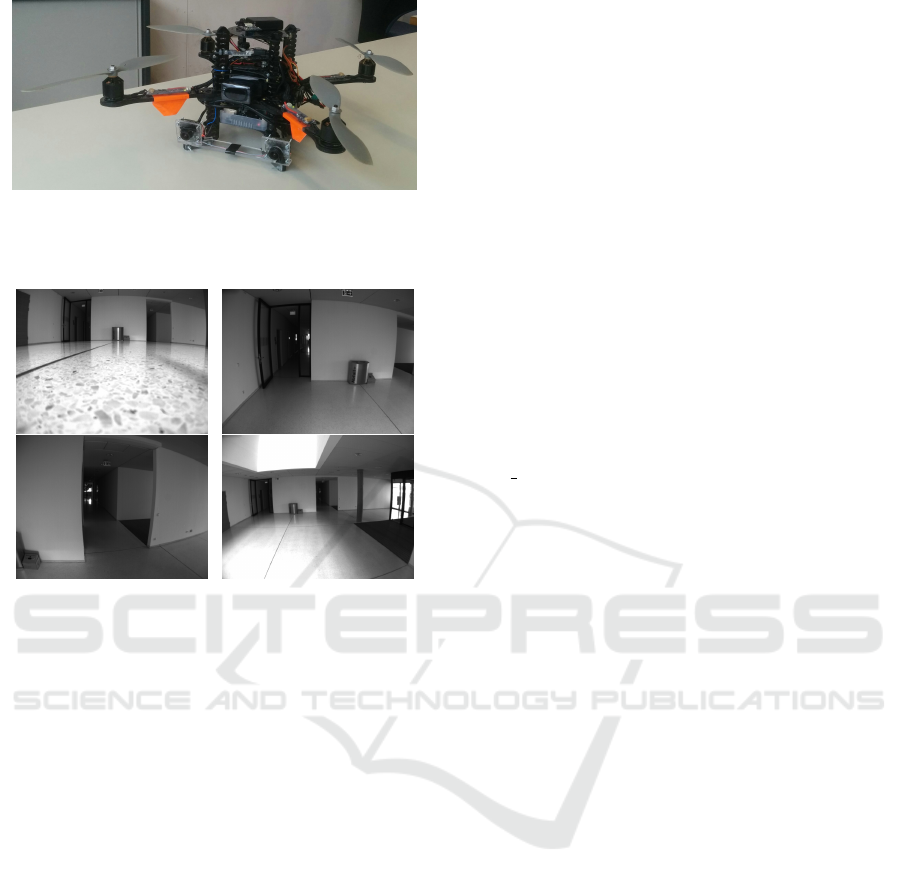
Figure 5: The Asctec Pelican used to acquire our own test
dataset. It is equipped with an IMU (included in the autopi-
lot), a stereo camera and an Odroid XU3 Lite processing
board.
Figure 6: Images of the sequence acquired with the flying
MAV. As can be seen, the scene mostly consists of white
walls with little texture.
absolute trajectory error can be observed. This sce-
nario is similar to an augmented reality application,
where, for example, an MAV equipped with a laser
projector should project something onto the wall.
As can be seen in the input images in Fig. 6,
the scene mostly consists of white, untextured walls.
Only few structure elements are visible (doors, recy-
cle bin).
We compare this sequence with Libviso (Geiger
et al., 2011) and LSD-SLAM (Engel et al., 2014). As
LSD-SLAM is a monocular approach and therefore
does not provide a metric scale, we manually aligned
the trajectory scale with the stereo approaches. How-
ever, generally this trajectory should be well suited for
a monocular approach, as there are no pure rotations
and no forward movement in the initialization phase.
The computed trajectories are plotted in Fig. 7. In
comparison to Libviso (blue), our approach (red) does
not have a big drift. The start/end point difference
of our approach is approximately 2.5 m while Lib-
viso has a difference of approximately 7 m. Libviso
has already a big translational drift when the MAV
is standing still on the floor at the beginning of the
trajectory. While flying, Libviso accumulates a big
rotational drift, which leads to big changes in the z-
dimension. Contrary, LSD-SLAM estimates parts of
the trajectory quite well. However, some random pose
jumps happen in the estimation, which yields to a tra-
jectory which is partly far away from the correct so-
lution. In total, our approach performs best compared
to the others, as it does not have a big drift and no big
outliers.
4.4 Rawseeds
The Rawseeds datasets (Bonarini et al., 2006) (Ceri-
ani et al., 2009) are publicly available indoor and out-
door datasets captured with a ground robot equipped
with multiple sensors. Additionally, ground truth data
was captured for some parts of the trajectories with an
external tracking system.
In our experiments, we chose to use the Bic-
occa 2009-02-27a dataset, which is an indoor dataset
captured in a static environment with mixed natural
and artificial lightning. Note that this is a really large-
scale dataset, as the total trajectory length is 967.18
m. We used the left and right images of the trinocular
forward-looking camera for our experiments, which
have a resolution of 640x480 pixels each, a baseline
of 18 cm and were captured with 15 FPS. As the im-
ages were acquired roughly aligned with the grav-
ity direction, no IMU measurements are needed for
our algorithm. Example input images can be seen in
Fig. 8.
As the ground truth computed with an external
tracking system does not cover the whole trajectory,
we use the (publicly available) extended ground truth
in our experiments. This ground truth also includes
trajectory parts estimated with data of an onboard
laser scanner.
In the experiments for this dataset, we compare
our approach with Libviso. In Tab. 1 one can see
the relative pose errors as proposed in (Sturm et al.,
2012). Our approach gives better results for all com-
puted relative pose errors. However, due to the dif-
ficulty of the sequence, which also contains images
with no texture at all (see Fig. 8), the error is also rel-
atively high when using our algorithm. Additionally,
the framerate should be higher for our approach. As
this dataset is just captured with 15 FPS, sometimes
the scene just moves too fast in front of the camera
and the camera pose cannot be tracked exactly. How-
ever, in the parts of the sequences where there exist
some vertical line structure (e.g. doors, windows or
shelves), our approach works better and therefore the
errors are lower.
Direct Stereo Visual Odometry based on Lines
483
−4 −2 0 2 4 6 8
−6
−4
−2
0
2
4
y (meters)
x (meters)
−4 −2 0 2 4 6 8
−6
−4
−2
0
2
4
y (meters)
x (meters)
−4 −2 0 2 4 6 8
−6
−4
−2
0
2
4
y (meters)
x (meters)
−4 −2 0 2 4 6 8
−7
−6
−5
−4
−3
−2
−1
0
1
2
3
4
z (meters)
x (meters)
Libviso
−4 −2 0 2 4 6 8
−7
−6
−5
−4
−3
−2
−1
0
1
2
3
4
z (meters)
x (meters)
Our Approach
−4 −2 0 2 4 6 8
−7
−6
−5
−4
−3
−2
−1
0
1
2
3
4
z (meters)
x (meters)
LSD-SLAM
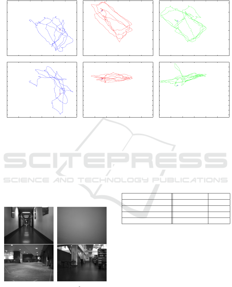
Figure 7: Estimated trajectories of Libviso (left, blue), our approach (middle, red) and LSD-SLAM (right, green) of the test
sequence captured with an MAV. Top row: x- and y-axes (top view). Bottom row: x- and z-axes (side view). The start point
is at (0,0,0) and the trajectory end point, which should be near the start point is indicated with a circle. Even though our
approach (red) has a slight drift (start point is not identical with end point), Libviso (blue) has a much higher rotational drift.
LSD-SLAM works well for some parts of the sequence. However, occasionally it does some random jumps and moves far
away from the desired trajectory.
4.5 KITTI
The KITTI dataset (Geiger et al., 2012) is currently a
popular dataset for visual odometry evaluation. It is
acquired with a stereo camera mounted on a car which
Figure 8: Images of the Rawseeds Bicocca 2009-02-27a se-
quence. Top left: A big part of the images look similar to
this, where the robot moves through a narrow corridor. Top
right: At some corridor intersections, where nearly pure ro-
tations are performed, just the white wall is captured with
the cameras, which is extremely difficult for a VO algorithm
Bottom row: Also parts with better input data for VO exist,
e.g., wider hallways and a library.
Table 1: Relative translational and rotational error of the
Rawseeds sequence as defined in (Sturm et al., 2012) per
seconds of movement of our approach and Libviso. In all
metrics, our approach performs better.
Our Approach Libviso
Transl. RMSE (m/s) 0.665 0.753
Transl. Median (m/s) 0.577 0.68
Rot. RMSE (deg/s) 10.892 12.229
Rot. Median (deg/s) 0.018 0.033
drives on public streets, mostly through cities. We
compare our algorithm against Libviso (Geiger et al.,
2011) on a subset of the dataset (sequence 07).
The images have a resolution of 1241x376 pixels
and a framerate of 10 FPS. As the images are roughly
aligned with the gravity direction, there is no need to
incorporate IMU measurements. Due to the low cap-
ture framerate and the relatively fast movement of the
car, the image content can change quite rapidly. This
is a problem for direct VO methods which deliver
good results when having small inter-frame motions.
Additionally, it contains enough texture for feature-
based methods to work properly. However, we want
to show that our approach works also well on datasets
for which it is not specifically designed for.
VISAPP 2016 - International Conference on Computer Vision Theory and Applications
484
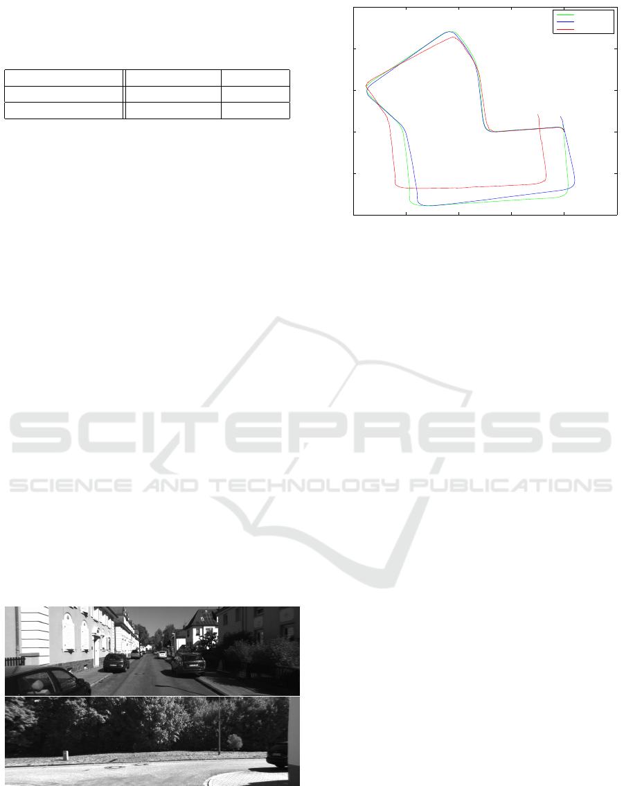
Table 2: Relative translational and rotational error of the
KITTI sequence 07 computed with the KITTI vision bench-
mark suite (Geiger et al., 2012) as mean over all possible
subsequences of length (100,...,800) meters.
Our Approach Libviso
Transl. error (%) 8.0558 2.3676
Rot. error (deg/m) 0.000744 0.000321
To overcome the low framerate, we had to change
the patch size of the patches around lines and points
used in the optimization from 21 to 31. Additionally,
we had to increase the maximal translational move-
ment for the optimization step. Using this settings
we get results comparable to state-of-the-art methods
with the drawback of higher runtimes compared to the
other datasets used in our evaluation. Additionally, as
more reliable points can be detected in this scene, we
decreased the line matching threshold so that more
points are used.
Also for Libviso, we changed the parameter set-
tings: We used it with default settings and subpixel
refinement.
In Fig. 10 the computed trajectories of Libviso and
our approach are plotted. As one can see, the abso-
lute trajectory error is slightly worse in our approach.
Also the rotational and translational errors as defined
in the KITTI vision benchmark suite are worse than
Libviso (see Tab. 2). However, our algorithm still
works acceptable on a dataset like this one for which
it is not designed for.
4.6 Runtime
The mean computation time per frame for the first
two datasets is 49.3 ms, which is a framerate of 20.3
FPS. With this computation speed, both the Rawseeds
Figure 9: Images of the KITTI visual odometry dataset (se-
quence 07). In this sequence, there are some lines detectable
in some parts (e.g. in top image). In these parts, the detected
lines are beneficial for the VO algorithm. However, in some
images there exist no lines (e.g. image bottom) and our al-
gorithm also depends on the detected feature points.
−200 −150 −100 −50 0 50
−100
−50
0
50
100
150
x (meters)
y (meters)
Ground Truth
Libviso
Our approach
Figure 10: Evolving trajectory of the KITTI sequence. One
can observe that our approach (red) performs comparable to
Libviso (blue).
dataset and our own MAV dataset can be processed in
real-time. Due to changed parameters for the KITTI
dataset, the computation speed for the KITTI dataset
is much slower and needs approximately 3 times the
processing time of the other datasets.
Most of the processing time is needed for the
pose estimation step, which could be optimized by a
multi-scale approach, using SIMD instructions (SSE,
NEON) or writing an own optimizer to overcome the
overhead of Ceres.
5 CONCLUSION
We have presented a direct stereo visual odometry
method, which detects and matches lines at every
keyframe using our novel fast line detection algorithm
and estimates the pose of consecutive frames by direct
pose estimation methods using patches around verti-
cal lines. These patches have proven to be a good
selection for indoor environments, which are poorly
textured, but where a lot of vertical structure exists.
In our experiments, we have shown that our algorithm
delivers better results than state-of-the-art methods in
challenging indoor environments and comparable re-
sults in well textured outdoor environments. As our
implementation runs in real-time, it is suitable for
various robotics and augmented reality applications.
Future work will include subpixel refinement of the
line detection step, global map optimization to mini-
mize drift errors and to evolve it to a complete SLAM
system, a multi-scale approach for the pose estima-
tion step to deliver better accuracy for large inter-
frame movements and improve computation speed,
and further speed improvements (e.g., using SSE and
Direct Stereo Visual Odometry based on Lines
485

NEON instructions) to make it real-time capable also
on small robotic platforms.
ACKNOWLEDGEMENTS
This project has been supported by the Austrian Sci-
ence Fund (FWF) in the project V-MAV (I-1537).
REFERENCES
Agarwal, S., Mierle, K., and Others. Ceres solver.
http://ceres-solver.org.
Bonarini, A., Burgard, W., Fontana, G., Matteucci, M., Sor-
renti, D. G., and Tardos, J. D. (2006). Rawseeds:
Robotics advancement through web-publishing of
sensorial and elaborated extensive data sets. In In-
ternational Conference on Intelligent Robots and Sys-
tems.
Ceriani, S., Fontana, G., Giusti, A., Marzorati, D., Mat-
teucci, M., Migliore, D., Rizzi, D., Sorrenti, D. G.,
and Taddei, P. (2009). Rawseeds ground truth collec-
tion systems for indoor self-localization and mapping.
Autonomous Robots, 27(4):353–371.
Cortinovis, A. (2010). Pixhawk - attitude and position
estimation from vision and imu measurements for
quadrotor control. Technical report, Computer Vision
and Geometry Lab, Swiss Federal Institute of Tech-
nology (ETH) Zurich.
Elqursh, A. and Elgammal, A. M. (2011). Line-based rel-
ative pose estimation. In Proceedings IEEE Confer-
ence Computer Vision and Pattern Recognition, pages
3049–3056. IEEE Computer Society.
Engel, J., Sch
¨
ops, T., and Cremers, D. (2014). Lsd-slam:
Large-scale direct monocular slam. In Proceedings
European Conference on Computer Vision.
Engel, J., St
¨
uckler, J., and Cremers, D. (2015). Large-scale
direct slam with stereo cameras. In International Con-
ference on Intelligent Robots and Systems.
Forster, C., Pizzoli, M., and Scaramuzza, D. (2014). Svo:
Fast semi-direct monocular visual odometry. In Inter-
national Conference on Robotics and Automation.
Furgale, P., Rehder, J., and Siegwart, R. (2013). Uni-
fied temporal and spatial calibration for multi-sensor
systems. In International Conference on Intelligent
Robots and Systems.
Geiger, A., Lenz, P., and Urtasun, R. (2012). Are we ready
for autonomous driving? the kitti vision benchmark
suite. In Proceedings IEEE Conference Computer Vi-
sion and Pattern Recognition.
Geiger, A., Ziegler, J., and Stiller, C. (2011). Stereoscan:
Dense 3d reconstruction in real-time. In IEEE Intelli-
gent Vehicles Symposion.
Grompone, R., Jakubowicz, J., Morel, J. M., and Randall,
G. (2010). Lsd: A fast line segment detector with a
false detection control. IEEE Transactions on Pattern
Analysis and Machine Intelligence, 32(4):722–732.
Hofer, M., Maurer, M., and Bischof, H. (2014). Improving
sparse 3d models for man-made environments using
line-based 3d reconstruction. In International Confer-
ence on 3D Vision.
Klein, G. and Murray, D. (2007). Parallel tracking and map-
ping for small ar workspaces. In Proceedings Interna-
tional Symposium on Mixed and Augmented Reality.
Levenberg, K. (1944). A method for the solution of certain
non-linear problems in least squares. In Quarterly of
Applied Mathematics 2, pages 164–168.
VISAPP 2016 - International Conference on Computer Vision Theory and Applications
486

Ma, Y., Soatto, S., Kosecka, J., and Sastry, S. S. (2003). An
Invitation to 3-D Vision: From Images to Geometric
Models. Springer Verlag.
Marquardt, D. (1963). An algorithm for least-squares esti-
mation of nonlinear parameters. In SIAM Journal on
Applied Mathematics 11(2), pages 431–441.
Mei, C., Sibley, G., Cummins, M., Newman, P., and Reid, I.
(2010). Rslam: A system for large-scale mapping in
constant-time using stereo. In International Journal
of Computer Vision.
Newcombe, R. A., Lovegrove, S. J., and Davison, A. J.
(2011). Dtam: Dense tracking and mapping in real-
time. In Proceedings International Conference on
Computer Vision, pages 2320–2327.
Rosten, E. and Drummond, T. (2005). Fusing points and
lines for high performance tracking. In Proceedings
International Conference on Computer Vision.
Sturm, J., Engelhard, N., Endres, F., Burgard, W., and Cre-
mers, D. (2012). A benchmark for the evaluation of
RGB-D SLAM systems. In International Conference
on Intelligent Robots and Systems, pages 573–580.
Weiss, S., Achtelik, M. W., Lynen, S., Achtelik, M. C.,
Kneip, L., Chli, M., and Siegwart, R. (2013). Monoc-
ular vision for long-term micro aerial vehicle state es-
timation: A compendium. Journal of Field Robotics,
30(5):803–831.
Direct Stereo Visual Odometry based on Lines
487
