High-dimensional Guided Image Filtering
Shu Fujita and Norishige Fukushima
Nagoya Institute of Technology, Nagoya, Japan
Keywords:
High-dimensional Filtering, Constant Time Filtering, Guided Image Filtering.
Abstract:
We present high-dimensional filtering for extending guided image filtering. Guided image filtering is one
of edge-preserving filtering, and the computational time is constant to the size of the filtering kernel. The
constant time property is essential for edge-preserving filtering. When the kernel radius is large, however, the
guided image filtering suffers from noises because of violating a local linear model that is the key assumption
in the guided image filtering. Unexpected noises and complex textures often violate the local linear model.
Therefore, we propose high-dimensional guided image filtering to avoid the problems. Our experimental
results show that our high-dimensional guided image filtering can work robustly and efficiently for various
image processing.
1 INTRODUCTION
Edge-preserving filtering has recently attracted at-
tention in image processing researchers. Such fil-
ters, e.g., bilateral filtering (Tomasi and Manduchi,
1998) and non-local means filtering (Buades et al.,
2005), are used for various applications including im-
age denoising (Buades et al., 2005), high dynamic
range imaging (Durand and Dorsey, 2002), detail en-
hancement (Bae et al., 2006; Fattal et al., 2007),
flash/no-flash photography (Petschnigg et al., 2004;
Eisemann and Durand, 2004), up-sampling/super res-
olution (Kopf et al., 2007), alpha matting (He et al.,
2010) and haze removing (He et al., 2009).
Edge-preserving filtering is often represented as
weighted averaging filtering by using space and color
distances among neighborhood pixels. When the dis-
tance is Euclidean, and the kernel weight is Gaus-
sian, this is a representative filter of the bilateral fil-
ter (Tomasi and Manduchi, 1998). The bilateral filter
has a number of acceleration methods (Porikli, 2008;
Yang et al., 2009; Paris and Durand, 2009; Pham
and Vliet, 2005; Fukushima et al., 2015). Domain
transform filtering (Gastal and Oliveira, 2011) and
recursive bilateral filtering (Yang, 2012), which use
geodesic distance, can also effectively filter images.
The guided image filter (He et al., 2010) is one
of the efficient edge-preserving filters; however, the
filtering property is different from the filters smooth-
ing with pixel-wise distance. The guided image fil-
ter assumes a local linear model in a kernel. Its
property is essential for several applications in com-
putational photography (Durand and Dorsey, 2002;
Petschnigg et al., 2004; Kopf et al., 2007; He et al.,
2010; He et al., 2009) and fast visual corresponding
problems (Hosni et al., 2013). The local linear model
is, however, violated by unexpected noises such as
Gaussian noises and multiple kinds of textures. Such
situation often happens when the size of the kernel is
large. Then, the resulting image may contain noises.
Figure 1 demonstrates feathering (He et al., 2010) and
the result of guided image filtering contains noises.
For efficient implementation, intensity/color in-
formation in each patch is gathered to channels or
dimensions in a pixel. Patch-wise processing is ef-
fective for handling the noisy information, e.g., non-
local means filtering (Buades et al., 2005) and DCT
denoising (Fujita et al., 2015). Then, the dimension of
the image becomes higher. The representation is ef-
ficiently smoothed as high-dimensional Gaussian fil-
tering (Adams et al., 2009; Adams et al., 2010; Gastal
and Oliveira, 2012; Fukushima et al., 2015). How-
ever, these filters do not have the similar property of
the guided image filtering for computational photog-
raphy. Figure 1 (e) shows the result by non-local
means filtering that is extended to joint filtering for
feathering. The result has been over-smoothed.
Therefore, we extend the guided image filtering
to store patch-wise neighborhood pixels into high-
dimensional space. We call this extension as high-
dimensional guided image filtering (HGF). We firstly
extend the guided image filtering to handle high-
dimensional signals. In this regard, letting d be the
number of dimensions of the guidance image, the
computational complexity is O(d
2.807···
) as pointed
in (Gastal and Oliveira, 2012). Therefore, we also
Fujita, S. and Fukushima, N.
High-dimensional Guided Image Filtering.
DOI: 10.5220/0005715100250032
In Proceedings of the 11th Joint Conference on Computer Vision, Imaging and Computer Graphics Theory and Applications (VISIGRAPP 2016) - Volume 3: VISAPP, pages 27-34
ISBN: 978-989-758-175-5
Copyright
c
 2016 by SCITEPRESS – Science and Technology Publications, Lda. All rights reserved
27

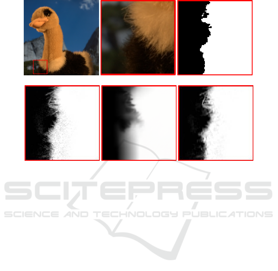
(a) Input (b) Guidance (c) Binary mask
(d) Guided image filtering (e) Non-local means (f) Ours (6-D)
Figure 1: Feathering results from guided image filtering (c) contains noises around object boundaries, while our result from
high-dimensional guided image filtering (d) suppresses such noises.
introduce a dimensionality reduction technique for
HGF to suppress the computational cost. Figure 1 (f)
indicates our result with reduced dimension.
2 RELATED WORKS
We discuss several acceleration methods of high-
dimensional filtering in this section.
The bilateral grid (Paris and Durand, 2009) is
used for color bilateral filtering whose dimension is
three. The dimension is not high; however, the sim-
ple regular grid is computationally inefficient; thus,
we use down-sampling of the grid for efficient filter-
ing. Note that the bilateral grid directly represents
the filtering space and is sparse. With this representa-
tion, the computational resource and the memory are
consumed beyond necessity. Due to this, the Gaus-
sian kd-trees (Adams et al., 2009) and the permuto-
hedral lattice (Adams et al., 2010) focus on represent-
ing the high-dimensional space with point samples.
These methods have succeeded to alleviate the com-
putational complexity when the filtering dimension is
high. However, since these works still require a sig-
nificant amount of calculation and memory, they are
not sufficiently for real-time applications.
The adaptive manifold (Gastal and Oliveira, 2012)
is a slightly different approach. The three methods de-
scribed above focus on how represents and expands
each dimension. By contrast, the adaptive manifold
samples the high-dimensional space at scattered man-
ifolds adapted to the input signal. Thus, we can
avoid enclosing pixels into cells to perform barycen-
tric interpolation. This property enables us to com-
pute a high-dimensional space efficiently and reduces
the memory requirement. The property is the rea-
son that the adaptive manifold is more efficient than
other high-dimensional filtering methods (Paris and
Durand, 2009; Adams et al., 2009; Adams et al.,
2010). On the other hand, the accuracy is lower than
them. The adaptive manifold causes quantization ar-
tifacts depending on the parameters.
3 HIGH-DIMENSIONAL GUIDED
IMAGE FILTERING
3.1 Definition
We extend guided image filtering (GF) (He et al.,
2010) for high-dimensional filtering in this section.
GF assumes a local linear model between an input
guidance image I
I
I and an output image q. The as-
VISAPP 2016 - International Conference on Computer Vision Theory and Applications
28

sumption of the local linear model is also invariant for
our HGF. Let J
J
J denote a n-dimensional guidance im-
age. J
J
J is generated from the guidance image I
I
I using
a function f :
J
J
J = f (I
I
I). (1)
The function f constructs a high-dimensional image
from I
I
I; for example, it uses a square neighborhood
centered at a pixel, discrete cosine transform (DCT)
or principle components analysis (PCA) of the guid-
ance image I
I
I.
HGF utilizes this high-dimensional image J
J
J as the
guidance image; thus, the output q is derived from a
linear transform of J
J
J in a square window ω
k
centered
at a pixel k . When we let p be an input image, the
linear transform is represented as follows:
q
i
= a
a
a
T
k
J
J
J
i
+ b
k
. ∀i ∈ ω
k
. (2)
Here, i is a pixel position, and a
a
a
k
and b
k
are linear
coefficients. In this regard, J
J
J
i
and a
a
a
k
represent n ×
1 vectors. Moreover, the linear coefficients can be
derived by the solution used in (He et al., 2010). Let
|ω| denote the number of pixels in ω
k
, and let U be
a n × n identical matrix. The linear coefficients are
computed by:
a
a
a
k
= (Σ
k
+ εU)
−1
(
1
|ω|
∑
i∈ω
k
J
J
J
i
p
i
− µ
µ
µ
k
¯p
k
) (3)
b
k
= ¯p
k
− a
a
a
T
k
µ
µ
µ
k
, (4)
where µ
µ
µ
k
and Σ
k
are the n × 1 mean vector and the
n×n covariance matrix of J
J
J in ω
k
, ε is a regularization
parameter, and ¯p
k
(=
1
|ω|
∑
i∈ω
k
p
i
) represents the mean
of p in ω
k
.
Finally, we compute the filtering output by apply-
ing the local linear model to all local windows in the
whole image. Note that q
i
in each local window in-
cluding a pixel i is not same. Therefore, the filter out-
put is computed by averaging all the possible values
of q
i
as follows:
q
i
=
1
|ω|
∑
k:i∈ω
k
(a
a
a
k
J
J
J
i
+ b
k
) (5)
=
¯
a
a
a
T
i
J
J
J
i
+
¯
b
i
, (6)
where
¯
a
a
a
i
=
1
|ω|
∑
k∈ω
i
a
a
a
k
and
¯
b
i
=
1
|ω|
∑
k∈ω
i
b
k
.
Computational time of HGF does not depend on
the kernel radius that is the inherent ability of GF.
HGF consists of many times of box filtering, which
can compute in O(1) time (Crow, 1984), and per-
pixel small matrix operations. However, the number
of times of box filtering linearly depends on the di-
mensions of the guidance image, and the order of the
matrix operations depend on exponentially in the di-
mensions.
3.2 Dimensionality Reduction
For efficient computing, we utilize PCA for dimen-
sionality reduction. The dimensionality reduction has
been proposed in (Tasdizen, 2008). The approach
aims for finite impulse response filtering using Eu-
clidean distance. In this paper, we adopt the technique
for HGF to extend GF.
For HGF, the guidance image J
J
J is converted to
new guidance information that is projected onto the
lower dimensional subspace determined by PCA. Let
Ω be a set of all pixel positions in J
J
J. To conduct PCA,
we should firstly compute the n×n covariance matrix
Σ
Ω
for the set of all guidance image pixel J
J
J
i
. The
covariance matrix Σ
Ω
is computed as follows:
Σ
Ω
=
1
|Ω|
∑
i∈Ω
(J
J
J
i
−
¯
J
J
J)(J
J
J
i
−
¯
J
J
J)
T
, (7)
where |Ω| and
¯
J
J
J are the number of all pixels and the
mean of J
J
J in the whole image, respectively. After
that, pixel values in the guidance image J
J
J are pro-
jected onto d-dimensional PCA subspace by the inner
product of the guidance image pixel J
J
J
i
and the eigen-
vectors e
e
e
j
(1 ≤ j ≤ d, 1 ≤ d ≤ n, where d is a con-
stant value) of the covariance matrix Σ
Ω
. Let J
J
J
d
be a
d-dimensional guidance image, then the projection is
performed as:
J
d
i j
= J
J
J
i
· e
e
e
j
, 1 ≤ j ≤ d, (8)
where J
d
i j
is the pixel value in the j-th dimension of
J
J
J
d
i
, and J
J
J
i
· e
e
e
j
represents the inner product of the two
vectors. We show an example of the PCA result of
each eigenvector e
e
e in Fig. 2.
In this way, we can obtain the d-dimensional guid-
ance image J
J
J
d
. This guidance image J
J
J
d
is used by re-
placing J
J
J in Eqs. (2), (3) (5) and (6). Moreover, each
dimension in J
J
J
d
can be weighed by the eigenvalues λ
λ
λ,
where is a d × 1 vector, of the covariance matrix Σ
Ω
.
Note that the eigenvalue elements from the (d + 1)-th
to n-th are discarded because HGF only use d dimen-
sions. Hence, the identical matrix U in Eq. (3) can be
weighted as to the eigenvalues λ
λ
λ. Then, we take the
element-wise inverse of the eigenvalues λ
λ
λ:
E
E
E
d
= U λ
λ
λ
inv
(9)
=



1
λ
1
.
.
.
1
λ
d



, (10)
where E
E
E
d
represents a d ×d diagonal matrix, λ
inv
rep-
resents the element-wise inverse eigenvalues, and λ
x
is the x-th eigenvalue. Note that we take the logarithm
of the eigenvalues λ
λ
λ as to applications and normalize
High-dimensional Guided Image Filtering
29

(a) Input (b) 1st dimension (c) 2nd dimension
(d) 3rd dimension (e) 4th dimension (f) 5th dimension
Figure 2: PCA result. We construct the color original high-dimensional guidance image from 3 × 3 square neighborhood in
each pixel of the input image. We reduce the dimension 27 = (3 × 3 × 3) to 5.
the eigenvalue based on the 1st eigenvalue λ
1
. Tak-
ing the element-wise inverse of λ
λ
λ is to use the small
ε for the dimension having the large eigenvalue as
compared to the small eigenvalue. The reason is that
the elements of λ
λ
λ satisfy λ
1
≥ λ
2
≥ · ·· ≥ λ
d
, and the
eigenvector whose eigenvalue is large is more impor-
tant. As a result, we can preserve the characters of the
image in the principal dimension.
Therefore, we can obtain the final coefficient
a
a
a
k
instead of using Eq. (3) in the case of high-
dimensional case as follows:
a
a
a
k
= (Σ
d
k
+ εE
E
E
d
)
−1
(
1
|ω|
∑
i∈ω
k
J
J
J
d
i
p
i
− µ
µ
µ
d
k
¯p
k
), (11)
where and µ
µ
µ
d
k
and Σ
d
k
are the d × 1 mean vector and
the d × d covariance matrix of J
J
J
d
in ω
k
.
4 EXPERIMENTAL RESULTS
In this section, we evaluate the performance of HGF
in terms of efficiency and also verify the characteris-
tics by using several applications. In our experiments,
0
5
10
15
20
25
5 10 15 20 25
Processing time (sec)
Guidance image dimension d
Grayscale
Color
1 3
Figure 3: Processing time of high-dimensional guided im-
age filtering with respect to guidance image dimensions.
each pixel of high-dimensional images J
J
J has multiple
pixel values that consist of a fixed-size square neigh-
borhood around each pixel in original guidance image
I
I
I. Note that the dimensionality is reduced by the PCA
approach discussed in Sec. 3.2.
We firstly reveal the processing time of HGF.
We have implemented our proposed and competi-
VISAPP 2016 - International Conference on Computer Vision Theory and Applications
30

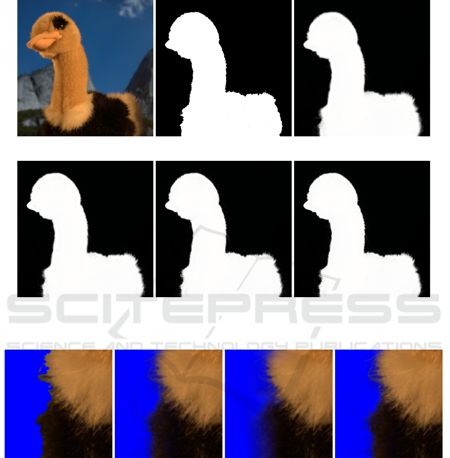
(a) Guidance image (b) Binary mask (c) 3-D HGF
(d) 6-D HGF (e) 10-D HGF (f) 27-D HGF
Figure 4: Dimension sensitivity. The color patch size for high-dimensional image is 3 × 3, i.e., the full dimension is 27. The
parameters are r = 15, ε = 10
−6
.
(a) Binary mask (b) GF (c) Non-local means (d) 6-D HGF
Figure 5: Matting result using alpha masks in Fig. 1.
tion methods written in C++ with Visual Studio 2010
on Windows 7 64 bit. The code is parallelized by
OpenMP. The CPU for the experiments is 3.50 GHz
Intel Core i7-3770K. The input images whose resolu-
tion is 1-megapixel, i.e., 1024 × 1024, are grayscale
or color images.
Figure 3 shows the result of the processing time.
The processing time of HGF exponentially increases
as the guidance image dimensionality becomes high.
From this cost increasing result, the dimensionality
reduction is essential for HGF. Also, the computa-
tional cost of PCA is small as compared with the in-
crease of the filtering time by increasing the dimen-
sionality. Therefore, although the computational cost
becomes high by increasing the dimensionality, the
problem is not significant. Tasdizen (Tasdizen, 2008)
also remarked that the performance of the dimension-
ality reduction peaks at around 6. The fact is shown
in following our experiments.
Figure 4 shows the result of the dimension sensi-
tivity of HGF. We can improve the edge-preserving
effect of HGF by increasing the dimension. The
High-dimensional Guided Image Filtering
31

(a) Input image (b) GF (c) 6-D HGF
(d) Detail of (b)
(e) Detail of (c)
Figure 6: Image abstraction. The local patch size for high-dimensional image is 3 × 3. The parameters for GF and HGF are
r = 25, ε = 0.04
2
.
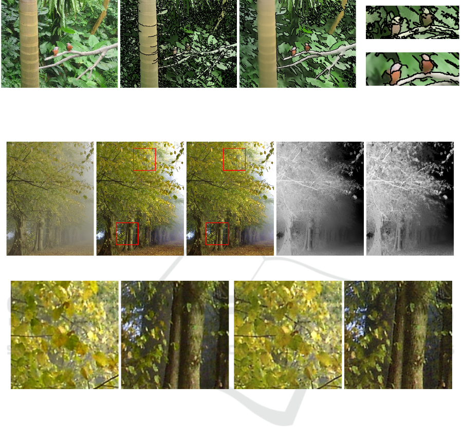
(a) Hazy image (b) GF (c) Ours (d) GF (e) Ours
(f) Detail of (b) (g) Detail of (c)
Figure 7: Haze removing. The bottom row images represent transition maps of (b) and (c). The local patch size for high-
dimensional image is 5 × 5. The parameters for GF and HGF are r = 20, ε = 10
−4
.
amount of the improvement is, however, slight in the
case of over 10-D. Thus, we do not need to increase
the dimension.
Next, we discuss the characteristics between GF
and HGF. As mentioned in Sec. 1, GF can transfer
detailed regions such as feathers, but it may cause
noises near the object boundary at the same time (see
Fig. 1 (d)). By contrast, HGF can suppress the noises
while the detailed regions are transferred as shown in
Fig. 1 (f).
We also show the results of alpha matting in Fig. 5.
The used alpha masks are shown in Figs. 1 (c)-(f).
The result of guided image filtering has noises and
color mixtures near the object boundary. The result
of non-local means filtering has the blurred edges.
These problems are solved in HGF. In our method,
the noises and color mixtures are reduced, the blur is
not caused.
Figure 6 shows the image abstraction results. Note
that the result takes 3 times iterations of filtering. As
shown in Figs. 6 (b) and (d), since the local linear
model is often violated in filtering with large kernel,
the pixel values are scattered. On the other hands,
HGF can smooth the image without such problem
(see Figs. 6 (c) and (e)).
HGF also has an excellent performance for haze
removing (He et al., 2009). The haze removing re-
sults and the transition maps are shown in Fig. 7. In
the case of GF, the transition map preserves major tex-
tures while there are over-smoothed regions near the
detailed regions or object boundaries, e.g., between
trees or branches. The over-smoothing effect affects
VISAPP 2016 - International Conference on Computer Vision Theory and Applications
32

(a) Example of spectral image (b) Grand truth
Corn-no till
Corn-min till
Corn
Soybeans-no till
Soybeans-min till
Soybeans-clean till
Alfalfa
Grass/pasture
Grass/trees
Grass/pasture-mowed
Hay-windowed
Oats
Wheat
Woods
Bldg-Grass-Tree-Drives
Stone-steel towers
(c) Labels
(d) SVM result (Melgani and
Bruzzone, 2004)
(e) GF (Kang et al., 2014) (f) 6-D HGF
Figure 8: Classification result of Indian Pines image. The image of (a) represents a spectral image that the wavelength is
0.7µm. The parameters for GF and HGF are r = 4, ε = 0.15
2
.
the haze removal in such regions. In our case, the
transition map of HGF preserves such detailed tex-
ture; thus, HGF can remove the haze better than GF
in detailed regions. For these results, HGF is effective
for preserving the detailed areas or textures.
As the other application for high-dimensional
guided image filtering, there is an image classifica-
tion with a hyperspectral image. The hyperspectral
image has various wavelength information, which is
useful for distinguishing different objects. Although
we can obtain a good result by using support vec-
tor machine classifier (Melgani and Bruzzone, 2004),
Kang et al. improved the accuracy of image classifi-
cation by applying guided image filtering (Kang et al.,
2014). They made a guidance image using PCA from
the hyperspectral image, but most of the informa-
tion was unused because GF cannot utilize the high-
dimensional data. Our extension has an advantage in
such case. Since HGF can utilize high-dimensional
data, we can further improve the accuracy of classifi-
cation by adding the unused information.
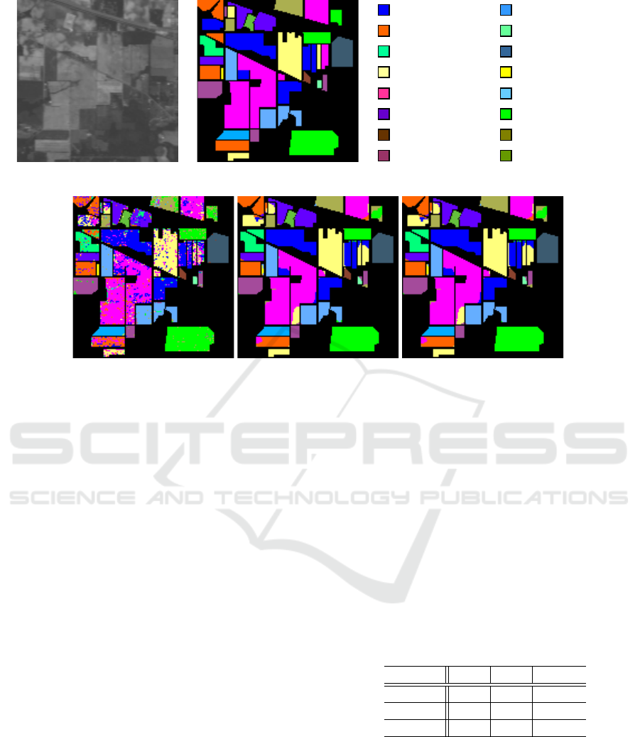
Figure 8 and Tab. 1 show the result of classifi-
cation of Indian Pines dataset, which was acquired
by Airborne Visible/Infrared Imaging Spectrometer
(AVIRIS) sensor. We objectively evaluate the classifi-
cation accuracy by using the three metrics: the overall
accuracy (OA), the average accuracy (AA), and the
kappa coefficient, which are widely used for evaluat-
ing classification. OA denotes the ratio of correctly
classified pixels. AA denotes the average ratio of cor-
rectly classified pixels in each class. The kappa coef-
ficient denotes the ratio of correctly classified pixels
corrected by the number of pure agreements. We can
confirm that the HGF result achieves the better result
than GF. Especially, the detailed regions are improved
in our method. The accuracy is objectively further im-
proved as shown in Tab. 1.
Table 1: Classification accuracy [%] of the classification
results shown in Fig. 8.
Method OA AA Kappa
SVM 81.0 79.1 78.3
GF 92.7 93.9 91.6
HGF 92.8 94.1 91.8
5 CONCLUSION
In this paper, we proposed high-dimensional guided
image filtering (HGF) by extending guided image fil-
tering (He et al., 2010). Due to this extension, guided
image filtering obtains the robustness for unexpected
noises such as Gaussian noises and multiple textures.
High-dimensional Guided Image Filtering
33

Also our method enable the guided image filter to ap-
ply for a high-dimensional image such as a hyper-
spectral image. HGF has a limitation that the compu-
tational cost becomes high by increasing the number
of dimensions. For this reason, we also introduce the
dimensionality reduction technique for efficient com-
puting. Experimental results showed that HGF can
work robustly in noisy regions and transfer detailed
regions. In addition, we can compute efficiently by
using the dimensionality reduction technique.
We construct the high-dimensional guidance im-
age from the square neighborhood in each pixel.
Therefore, as our future work, we consider the investi-
gation of the generating method for high-dimensional
guidance image.
ACKNOWLEDGEMENT
This work was supported by JSPS KAKENHI Grant
Number 15K16023.
REFERENCES
Adams, A., Baek, J., and Davis, M. A. (2010). Fast high-
dimensional filtering using the permutohedral lattice.
Computer Graphics Forum, 29(2):753–762.
Adams, A., Gelfand, N., Dolson, J., and Levoy, M. (2009).
Gaussian kd-trees for fast high-dimensional filtering.
ACM Trans. on Graphics, 28(3).
Bae, S., Paris, S., and Durand, F. (2006). Two-scale tone
management for photographic look. ACM Trans. on
Graphics, 25(3):637–645.
Buades, A., Coll, B., and Morel, J. M. (2005). A non-local
algorithm for image denoising. In Proc. IEEE Con-
ference on Computer Vision and Pattern Recognition
(CVPR).
Crow, F. C. (1984). Summed-area tables for texture map-
ping. In Proc. ACM SIGGRAPH, pages 207–212.
Durand, F. and Dorsey, J. (2002). Fast bilateral filtering
for the display of high-dynamic-range images. ACM
Trans. on Graphics, 21(3):257–266.
Eisemann, E. and Durand, F. (2004). Flash photography
enhancement via intrinsic relighting. ACM Trans. on
Graphics, 23(3):673–678.
Fattal, R., Agrawala, M., and Rusinkiewicz, S. (2007). Mul-
tiscale shape and detail enhancement from multi-light
image collections. ACM Trans. on Graphics, 26(3).
Fujita, S., Fukushima, N., Kimura, M., and Ishibashi, Y.
(2015). Randomized redundant dct: Efficient denois-
ing by using random subsampling of dct patches. In
Proc. ACM SIGGRAPH Asia Technical Briefs.
Fukushima, N., Fujita, S., and Ishibashi, Y. (2015). Switch-
ing dual kernels for separable edge-preserving fil-
tering. In Proc. IEEE International Conference on
Acoustics, Speech and Signal Processing (ICASSP).
Gastal, E. S. L. and Oliveira, M. M. (2011). Domain
transform for edge-aware image and video processing.
ACM Trans. on Graphics, 30(4).
Gastal, E. S. L. and Oliveira, M. M. (2012). Adaptive man-
ifolds for real-time high-dimensional filtering. ACM
Trans. on Graphics, 31(4).
He, K., Shun, J., and Tang, X. (2010). Guided image ffil-
tering. In Proc. European Conference on Computer
Vision (ECCV).
He, K., Sun, J., and Tang, X. (2009). Single image haze
removal using dark channel prior. In Proc. IEEE Con-
ference on Computer Vision and Pattern Recognition
(CVPR).
Hosni, A., Rhemann, C., Bleyer, M., Rother, C., and
Gelautz, M. (2013). Fast cost-volume filtering for vi-
sual vorrespondence and beyond. IEEE Trans. on Pat-
tern Analysis and Machine Intelligence, 35(2):504–
511.
Kang, X., Li, S., and Benediktsson, J. (2014). Spectral-
spatial hyperspectral image classification with edge-
preserving filtering. IEEE Trans. on Geoscience and
Remote Sensing, 52(5):2666–2677.
Kopf, J., Cohen, M., Lischinski, D., and Uyttendaele, M.
(2007). Joint bilateral upsampling. ACM Trans. on
Graphics, 26(3).
Melgani, F. and Bruzzone, L. (2004). Classification of hy-
perspectral remote sensing images with support vector
machines. IEEE Trans. on Geoscience and Remote
Sensing, 42(8):1778–1790.
Paris, S. and Durand, F. (2009). A fast approximation of
the bilateral filter using a signal processing approach.
International Journal of Computer Vision, 81(1):24–
52.
Petschnigg, G., Agrawala, M., Hoppe, H., Szeliski, R., Co-
hen, M., and Toyama, K. (2004). Digital photography
with flash and no-flash image pairs. ACM Trans. on
Graphics, 23(3):664–672.
Pham, T. Q. and Vliet, L. J. V. (2005). Separable bilat-
eral filtering for fast video preprocessing. In Proc.
IEEE International Conference on Multimedia and
Expo (ICME).
Porikli, F. (2008). Constant time o(1) bilateral filtering. In
Proc. IEEE Conference on Computer Vision and Pat-
tern Recognition (CVPR).
Tasdizen, T. (2008). Principal components for non-local
means image denoising. In Proc. IEEE International
Conference on Image Processing (ICIP).
Tomasi, C. and Manduchi, R. (1998). Bilateral filtering for
gray and color images. In Proc. IEEE International
Conference on Computer Vision (ICCV).
Yang, Q. (2012). Recursive bilateral filtering. In Proc. Eu-
ropean Conference on Computer Vision (ECCV).
Yang, Q., Tan, K. H., and Ahuja, N. (2009). Real-time o(1)
bilateral filtering. In Proc. IEEE Conference on Com-
puter Vision and Pattern Recognition (CVPR).
VISAPP 2016 - International Conference on Computer Vision Theory and Applications
34