Learning T2D Evolving Complexity from EMR and Administrative

Data by Means of Continuous Time Bayesian Networks

Simone Marini, Arianna Dagliati, Lucia Sacchi

and Riccardo Bellazzi

Biomedical Informatics Labs “Mario Stefanelli”, Dept. of Electrical, Computer and Biomedical Engineering,

University of Pavia, Pavia, Italy

Keywords: Type 2 Diabetes, Continuous Time Bayesian Network, Cohort Modeling, Disease Complexity.

Abstract: Predicting the complexity level (i.e. the number of complications and their related hospitalizations) in a T2D

cohort is a critical step in prevention, resource optimization and overall patient management. Our data set

was obtained by monitoring a T2D diabetic cohort along up to 10 years through electronic medical records

of a local healthcare agency data warehouse. In order to conveniently handle temporarily sparse data, we

designed a model describing the cohort evolution with Continuous Time Bayesian Networks (CTBN). The

network structure and its parameters are entirely data driven. Compared to traditional Bayesian Networks,

CTBNs admit cycles. As consequence, CTBNs fit the complexity of chronic metabolic syndromes where

variables show a reciprocal influence. Network nodes represent metabolic (glycated hemoglobin, lipid

profile (cholesterol, triglycerides), and biometric (BMI) data. We observed how these variables directly or

indirectly affect the disease level of complexity, and how the variables influence the cumulative adverse

events a patient undergoes.

1 INTRODUCTION

The development of computational tools to support

decisions in Medicine is driven by the increasing

burden of health care costs. Simulation models are

viable tools to predict health outcomes in target

populations and thus help optimizing resources

(Tarride et al., 2010; Marini et al., 2015). Diabetes is

a disease affecting a growing number of patients,

387 million individuals in 2014 with up to 592

million patients estimated by 2035 (International

Diabetes Federation, 2014; McEwan et al., 2014).

Providing tools to help clinicians assessing the

evolution of a diabetic cohort over time can

therefore help manage the high costs of diabetes.

The EU funded Mosaic project is dedicated to

the development of several models able to depict

meaningful clinical pathways in Type 2 Diabetes

(T2D) patients, in order to understand which clinical

and exogenous factors trigger worsened patients'

profiles. The dataset collected in a first project phase

is made up of 1020 T2D patients. These retrieved

information include data from hospital electronic

medical records (EMR) merged with administrative

information coming from Local Health Care Agency

(Dagliati et al 2014a). This means that observations

about patients are retrieved from follow-ups, which

usually occur every 6 month near the hospital where

subjects are in treated, and depict how metabolic

control and lipid profile evolve during the 5 to 10

years observation period. Clinicians record the

arising of complications due to the chronic diseases.

A complication is tied to its detection through a

set of prescribed exams and not to its physiological

onset specifically. This fact shows the importance of

the jointly analysis of clinical interventions and

physiological processes. To reach a comprehensive

understanding of the evolution of the disease we

leverage on the data coming from Local Health Care

Agency that include hospitalizations, drug purchases

and ambulatory encounters. Merging those sources

of data represents the first step to assess the disease

progression from both health care and management

points of view.

The exploitation of data mining methods allows

to automatically detect and reconstruct the most

frequent clinical temporal pathways patients

underwent (Dagliati et al. 2014b).

Since patient data streams are scattered along a

ten-year timeline, we decided to apply Continuous

Time Bayesian Networks (CTBN) (Nodelman and

al. 2002a) to design a network modelling TD2

338

Marini, S., Dagliati, A., Sacchi, L. and Bellazzi, R.

Learning T2D Evolving Complexity from EMR and Administrative Data by Means of Continuous Time Bayesian Networks.

DOI: 10.5220/0005708103380344

In Proceedings of the 9th International Joint Conference on Biomedical Engineering Systems and Technologies (BIOSTEC 2016) - Volume 5: HEALTHINF, pages 338-344

ISBN: 978-989-758-170-0

trajectories. CTBNs have been successfully

exploited in Medicine (Gatti et al., 2012, Wang et

al., 2014) and Bioinformatics (Acerbi and Stella

2014, Liu et al., 2009).

2 METHODS

2.1 Variable Discretization

Firstly we have selected from the Mosaic data base a

set of meaningful clinical variables able to

characterize multiple aspects in the patients’ cohort:

metabolic control (hba1c), lipid profile (cholesterol

and triglycerides) and weight changes (BMI). All the

listed variables are relevant in T2D treatment and

control (American Diabetes Association, 2013;

Solano et al., 2006).

We defined the possible node states through

physiological parameters discretization. Discrete

states start from 0, with increasing values indicating

a progressive worsening of the patient condition. To

discretize variables, we used fixed threshold defined

by the Italian clinical guidelines for T2D care

(http://www.aemmedi.it/). Table 1 shows the states

and discretization thresholds of clinical variables.

Table 1: Number of states and discretization thresholds of

clinical variables.

Node’s state 0 1 2

HBA1c (mmol/mol) <59 ≥59 -

BMI <20 [20, 30] >30

CHOLESTEROL

(mg/dl)

<220

[220,

280]

≥280

TRIGLYCERIDES

(mg/dl)

<170

[170,

350]

≥350

Complications are tracked by worsening patient

condition and health care services accesses. Most of

the cost associated with diabetes is related to the

management of these complications (McEvan et al.,

2014). To assess the patient care complexity over

time, we defined a set of four complexity stages

(LOC, Level of Complexity) determined by the

number of complications and hospitalizations a

patient undergoes. Higher complexity means a

higher need for resources and a higher cost to

manage him/her (increased hospitalization rate,

more need for specific examinations, etc.). LOC is

an analytic indication of disease complexity

allowing to summarize the overall patient condition

in single number. We have defined complexity

levels and related status of network nodes as

follows.

STATUS 0: Stable patients. This segment belongs to

pre-diabetic patients and T2D patients not suffering

any complication yet.

STATUS 1: 1st level of complexity. Patients who are

starting to develop the first complication and require

punctual treatments. This stage and the following

one are built upon clinicians notes in the hospital

Electronic Medical Record (EMR). Complications

include Macro vascular event (i.e. Acute Myocardial

Infarction, Angina, Chronic ischemic heart disease,

Occlusion and stenosis of carotid artery, Peripheral

vascular disease, Stroke), Micro vascular event (i.e.

Diabetic Foot, Nephropathy, Retinopathy) and Not

Vascular event (i.e. Neuropathy, Fatty Liver

Disease).

STATUS 2: 2nd level of complexity. Patients with

multiple complications that need to be followed by

more than one specialist on a frequent basis.

STATUS 3: 3rd level of complexity. Patients likely

to suffer hospitalizations either due to the status of

their diabetes-related complications or because of

their metabolic instability. This stage triggers when

a previously developed complication leads to a

hospitalization that is detected through the

administrative data stream. Associations between

complications and hospital accesses have been

settled thanks to the collaboration with clinicians

(e.g. a hospitalization where the principal diagnosis

has been recorded with an IC9 code indicating a

disease of the genitourinary system after the onset of

Nephropathy).

2.2 Data Pre-processing and Data Set

Building

A first issue that we considered while analysing data

coming from a hospital EMR together with

administrative information is that T2D patients do

not start to be followed at the hospital immediately

after diabetes diagnosis. This happens because this

type of chronic patients are initially in charge of

their general practitioners who manage their cure

until it is more suitable for them to be followed in a

centre specialized in diabetes treatment.

For this reasons, observations do not show an

initial common time stamp, and some variables are

measured more frequently than other. Moreover,

these timestamps may vary also because of changes

in the patient conditions. For each time point we

have a direct observation for one or two variables

(e.g. cholesterol and triglycerides are often measured

together), but we lack information about unobserved

ones. Consequently, temporally sparse data with

Learning T2D Evolving Complexity from EMR and Administrative Data by Means of Continuous Time Bayesian Networks

339

missing values need to be pre-processed in order to

create suitable samples to be analysed with CTBNs

(e.g., the state of a variable was propagated until the

next known/measured value).

2.3 CTBN Machinery

Temporal dynamics are represented explicitly in

CTBNs. The system state space evolution is

described through conditional intensity matrices

(CIM) (Nodelman et al., 2002a). The number of

CIMs for each node is equivalent to the possible

state combinations of its parent nodes. For example,

if a child node C

has a parent node P

, and P

has

two states, then node C

is described by two CIMs.

If a child node C

has two parent nodes P

and P

with two and three states respectively, then C

described by six CIMs. CIMs are utilized to simulate

the evolution of the network state. Each CIM is a

square matrix, with a row for each state of the

described node, according the following schema:

CIM(C|p)

1(p)

12(p)

… q

1m(p)

21(p)

-q

2(p)

… q

2m(p)

…

… …

m1(p)

m2(p)

… -q

m(p)

The schema represents a CIM for the node C,

where p is the parent node status and m is the

number of states of C. In the example above, it could

be for instance P

=0 and P

=2. The elements q

the principal diagonal are related to the transition

time. In particular, when a node switches to the i-th

state, we utilize -q

to compute the time the node will

take before switching again. The time a node

remains in its state is randomly draw from an

exponential distribution with parameter q

, 



∗









∗



, t ≥ 0.

Elements q

not belonging to the principal

diagonal are always > 0 and they are utilized to

compute the next node state. Once a transition

happens (i.e. the time sampled by the distribution

above is expired), the node switches to another state

with probability









Note that for each row with m elements,

∑







For example, if the first row a 3×3 CIM is [20 15

5], then the modeled node has three states, and the

first row models the behavior of the node in the first

state; the node remains in the first state for a time

sampled by a distribution with parameter 





20. Once the node switches, it randomly ends in

the second state with probability 15/20 = 0.75, and

to the third state with probability 5/20 = 0.25.

To implement or CTBN, we utilized R Package

for Continuous Time Bayesian Networks (Shelton et

al., 2010).

2.4 Network Learning

The problem of learning the structure of a CTBN

from a data set D can be tackled as the problem of

finding a structure G maximizing a Bayesian score

(Nodelman et al., 2002b):

score



G∶D



ln









ln

While this problem is NP-hard in traditional

Bayesian Networks, it has been shown (Nodelman et

al., 2002b) that in CTBN it is possible to optimize

the parent set for each variable of the CTBN

independently. In other words, we can explore the

parent space of each variable with a local search to

find the best score. Once the maximum number of

parents local search is fixed, the search is

polynomial with respect to the number of variables

and the size of the data set (Nodelman et al., 2002b).

The aforementioned Bayesian score can be

decomposed in a sum of local contribution (i.e.

family scores). Each local score assess the quality of

a given putative parent set of a single variable. In

this way, we can optimize the parent set of each

variable taken singularly. For a more detailed

explanation of this process, we address the reader to

works of Nodelman (Nodelman et al., 2002a;

Nodelman et al., 2002b).

Note that no parameters had to be tuned for the

learning phase.

3 RESULTS

3.1 Network Structure

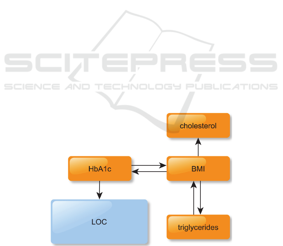
The resulting CTBN is shown in Figure 1. While the

only node directly affecting LOC is hbA1c, it is also

important to note that all the other nodes, with the

exception of cholesterol, are indirectly connected to

LOC through BMI and HbA1c. This means that the

model accounts for a wide variety of variables to

simulate the evolution of LOC. In other words, the

CTBN successfully learn meaningful variables

interconnections. HbA1c is a marker of long term

blood glucose concentration control, thus having a

pivotal role in diabetes monitoring.

Our network mimics how short-term changing

HEALTHINF 2016 - 9th International Conference on Health Informatics

340

variables (BMI influencing cholesterol and

triglycerides, and being influenced by triglycerides)

on the long run may raise the HbA1c level, which is

the key factor in determining the LOC and thus the

patient general health. In our learned network,

cholesterol does not influence LOC or any other

node. This does not mean cholesterol do not play a

role in the diabetes machinery, but rather than its

role does not emerge from our data.

3.2 Available Data Amount Influences

the Learned Network Structure

We assessed how the amount of available data

affects the network learning. We iteratively removed

an increasing number of random patient samples and

compared the learned network structure to the one

obtained from the full data set. In particular, we

gradually reduced our dataset by randomly removing

5% of the patients, and eventually reaching 50% of

the original data after 10 steps. We repeated 100

times this 10 step procedure, and we measured at

each step (a) if the network structure matches the

one learned on the full data set; and (b) the number

of the network edges of the newly learned network.

Results are shown in Figures 2 and 3.

Considering Figure 2, the amount of data seems

to be critical for this network design only when the

number of patients is less than 85% (~800 patients).

This means the very same network structure

emerges from data even if we remove 15% of the

available patients from our study (more than 95% of

the newly learned networks overlap the original).

This suggests the learned structure describes T2D

diabetes trajectories in a general and robust way.

However, this overlapping structure percentage

quickly drops once we utilize 75% or less of the

available patients. Similarly, as shown in Figure 3,

the edge number is reduced when fewer patients are

utilized for learning, leading to less rich and

interconnected networks.

3.3 Simulating LOC

We run a ten years long simulation with our

network. In particular, for each real patient, ten

artificial patients were simulated. Keeping a one-day

pace, the percentage of real (Rp) and simulated

patients (Sp) in a given LOC state were measured. It

was thus possible to calculate a daily LOC per-state

error as

  

, where



is the absolute value of

. The errors are depicted in Figure 4 with the blue

line. In general, we observed that the error grows

over time, but it is mostly below 15%. In fact, it is

always <10% for LOC 0, and it grows over 20%

only for LOC 1 after about three thousand days (thus

more than eight years after the beginning of the

simulation). Note that the granularity of the

simulation depends on the available data. In fact, in

CTBN we can simulate a step as short as the shortest

time unit utilized to measure our data. This means

that, since our EMR reported the date the patients

were visited and their data were recorded, we could

run simulations with a one day pace.

In order to validate our analysis, we proceeded

by randomly splitting our data into a training (85%)

and a test set (15%). We then re-learned the network

as from the training set only (the structure was

unaltered) and simulated the evolution of the learned

network for 10 years. The errors are measured as

explained above and depicted in Figure 4 with the

grey line. As expected, the errors on the test set were

higher, but still in a reasonable range, and below

25%.

4 CONCLUSIONS

In this work we designed a CTBN to describe a T2D

cohort. CTBN learning produced a meaningful

network fitting medical literature. Simulations

confirm that even for a ten year long timespan, error

in LOC is kept reasonably low (below 25%).

Moreover, the network is stable and it emerges from

data even if we remove 15% of the patient samples.

Although we obtained clinically meaningful

results, we are aware of some possible weakness in

this current approach. These weak aspects are

mainly related to the pre-processing of variable, like

Age or Time from Diagnosis, which naturally

increase during time. We are currently enhancing the

algorithm in order to make it able to process these

kinds of variables, taking into account that their

probability to change over time does not depend on

exogenous factors but it is intrinsic.

Furthermore, in future works, we aim to expand

our approach by including more network variables.

In particular, we will integrate EMR data with

administrative data about drug purchases to study

how different type of drugs (like Diabetes Therapies,

Antihypertensive and Statins) might cast an

influence on LOC.

REFERENCES

Acerbi, E., Stella, F. 2014. Continuous Time Bayesian

Networks for Gene Network Reconstruction: A

Learning T2D Evolving Complexity from EMR and Administrative Data by Means of Continuous Time Bayesian Networks

341

Comparative Study on Time Course Data.

Bioinformatics Research and Applications. Springer

International Publishing, 176-187.

American Diabetes Association 2013. Standards of

medical care in diabetes. Diabetes Care 36 (1): S11-

S66.

Dagliati, A., Sacchi, L., Bucalo, M., Segagni, D.,

Zarkogianni, K., Martinez Millana, A., Cancela, J.,

Sambo, F., Fico, G., Meneu Barreira, M.T., Cerra, C.,

Nikita, K., Cobelli, C., Chiovato, L., Arredondo, M.T.,

Bellazzi, R. 2014a. A Data Gathering Framework to

Collect Type 2 Diabetes Patients Data. Biomedical

and Health Informatics (BHI), 2014 IEEE-EMBS

International Conference Proceedings. 244 – 247.

Dagliati A., Sacchi, L., Cerra, C., Leporati, P., De Cata, P.,

Chiovato, L., Holmes, J.H., Bellazzi, R. 2014b.

Temporal Data Mining and Process Mining

Techniques to Identify Cardiovascular Risk-

Associated Clinical Pathways in Type 2 Diabetes

Patients Biomedical and Health Informatics (BHI),

2014 IEEE-EMBS International Conference

Proceedings. 240 – 243.

Gatti, E., Luciani, D., Stella, F. 2012. A continuous time

Bayesian network model for cardiogenic heart failure.

Flexible Services and Manufacturing Journal 4(4),

496—515.

International Diabetes Federation. 2014. IDF Diabetes

Atlas. 6th edn, 2014 Update. Brussels, Belgium:

International Diabetes Federation.

Liu, B., Thiagarajan, P.S., Hsu, D. 2009. Probabilistic

Approximations of Signaling Pathway Dynamics.

Computational Methods in Systems Biology. Springer

Berlin Heidelberg.

McEwan, P., Foos, V., Palmer, J.L., Lamotte, M., Lloyd,

A., Grant, D. 20014. Validation of the IMS CORE

Diabetes Model. Value Health (6):714-24.

Marini, S., Trifoglio, E., Barbarini, N., Sambo, F., Di

Camillo, B., Malovini, A., Manfrini, M., Cobelli, C.,

Bellazzi, R. 2015. A Dynamic Bayesian Network

model for long-term simulation of clinical

complications in type 1 diabetes. Journal of

Biomedical Informatics, ePub ahead of print.

Nodelman, U., Shelton, C.R., Koller, D. 2002a.

Continuous time bayesian networks. UAI02

Proceedings, 378—387.

Nodelman, U., Shelton, C.R., and Koller, D. 2002b.

Learning continuous time bayesian networks. In Proc.

of the 19th Conf. on Uncertainty in Artificial

Intelligence, pages 451–458.

Shelton, C.R., Fan, Y., Lam, W., Lee, J., Xu. J. 2010.

Continuous Time Bayesian Network Reasoning and

Learning Engine. The Journal of Machine Learning

Research 11: 1137-1140.

Solano, M.P., Goldberg, R.B. 2006. Lipid management in

type 2 diabetes. Clinical Diabetes 24(1): 27-32.

Tarride, J.E., Hopkins, R., Blackhouse, G., Bowen, J.M.,

Bischof, M., Von Key-serlingk, C., O’Reilly, D., Xie,

F., Goeree, R. 2010. A review of methods used in long-

term cost-effectiveness models of diabetes mellitus

treatment. Pharmacoeconomics. 28(4):255-77.

Wang, X., Sontag, D., Wang, F. 2014. Unsupervised

Learning of Disease Progression Models. Proceedings

of the 20th ACM SIGKDD international conference

on knowledge discovery and data mining, 85-94.

APPENDIX

Figure 1: The learned CTBN network.

HEALTHINF 2016 - 9th International Conference on Health Informatics

342

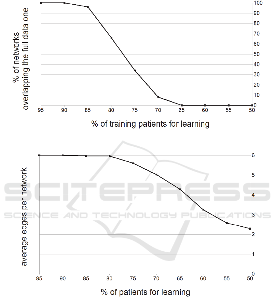
Figure 2: Percentage of newly learned network overlapping with the original one depends on the number of patients

sampled from the original data set.

Figure 3: Average edges per learned network depends on the fraction of patients sampled from the original data set.

Learning T2D Evolving Complexity from EMR and Administrative Data by Means of Continuous Time Bayesian Networks

343

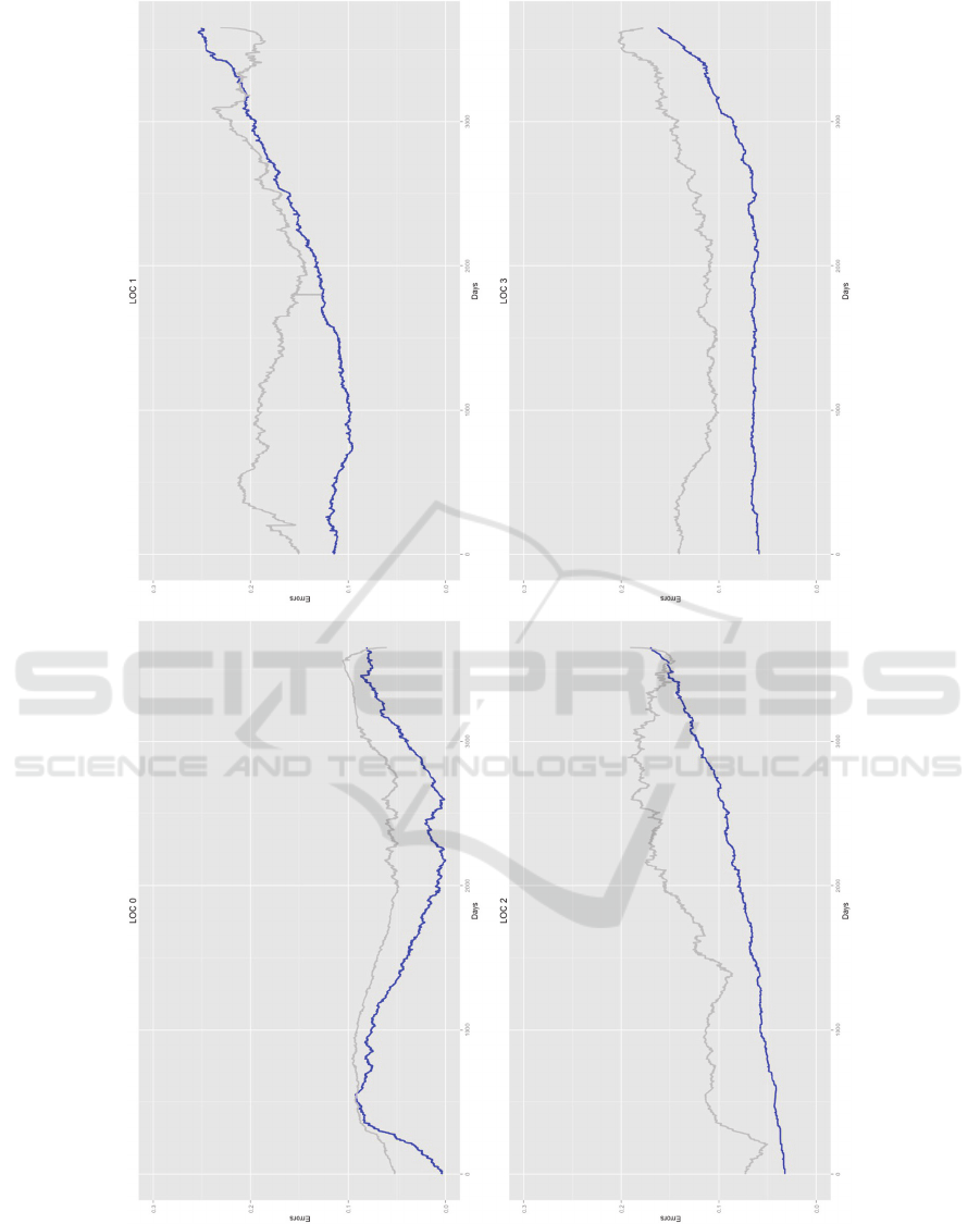
Figure 4: Error for each state of LOC node. Error is measured as the absolute difference between the amount of real and

simulated patients in a given state, at a given time (one day pace). The error utilizing all data is represented in blue, while

the error on a test set (not utilized for training) is in grey.

HEALTHINF 2016 - 9th International Conference on Health Informatics

344