
A Sampling Approach for Multiple RNA Interaction
Finding Sub-optimal Solutions Fast
Saad Mneimneh
1,∗
and Syed Ali Ahmed
2,†
1
Department of Computer Science, Hunter College of the City University of New York, New York, U.S.A.
2
Department of Computer Science, The Graduate Center of the City University of New York, New York, U.S.A.
Keywords:
Multiple RNA Interaction, RNA Structure, Gibbs Sampling, Metropolis-Hastings Algorithm, Clustering.
Abstract:
The interaction of two RNA molecules involves a complex interplay between folding and binding that war-
ranted recent developments in RNA-RNA interaction algorithms. These algorithms cannot be used to predict
interaction structures when the number of RNAs is more than two. Our recent formulation of the multiple
RNA interaction problem is based on a combinatorial optimization called Pegs and Rubber Bands, and has
been successful in predicting structures that involve more than two RNAs. Even then, however, the optimal
solution obtained does not necessarily correspond to the actual biological structure. Moreover, a structure
produced by interacting RNAs may not be unique to start with. Multiple solutions (thus sub-optimal ones)
are needed. We extend our previous approach to generate multiple sub-optimal solutions that was based on
exhaustive enumeration. Here, a sampling approach for multiple RNA interaction is developed. Since not too
many samples are needed to reveal solutions that are sufficiently different, sampling provides a much faster
alternative. By clustering the sampled solutions, we are able to obtain representatives that correspond to the
biologically observed structures. Specifically, our results for the U2-U6 complex and its introns in the spliceo-
some of yeast, and the CopA-CopT complex in E. Coli are consistent with published biological structures.
1 INTRODUCTION
The role of interaction between two or more RNA
molecules has been increasingly recognized in regula-
tory mechanisms, including gene expression, methy-
lation, and splicing. Pairwise interaction has been
noted for regulating gene expression, e.g. when one
RNA binds to the ribosome binding site of another
mRNA, thus blocking its translation to protein. Typi-
cal scenarios of multiple RNA interaction involve the
interaction of multiple small nucleolar RNAs (snoR-
NAs) with ribosomal RNAs (rRNAs) in guiding the
methylation of the rRNAs (Meyer, 2008), and multi-
ple small nuclear RNAs (snRNA) with mRNAs in the
splicing of introns (Sun and Manley, 1995).
The prediction of structures resulting from pair-
wise interactions is now somewhat understood, due
to successful efforts in generalizing the energy model
of a single RNA to the case of two. The partition
function Z of a single RNA is key in determining the
probability of structures.
∗
Partially supported by CoSSMO at CUNY.
†
Supported by a PSC CUNY Award 68671-00 46.
Z =
∑
S
e
−βE(S)
where S is a structure, E(S) is its free energy, and β
is typically 1/RT , where R is the Boltzman constant
and T is temperature. The probability of a structure S
is then given by:
P(S) =
e
−βE(S)
Z
and the probability of an event (e.g. the event
f ree[i, j] that bases i,i + 1,. .., j do not bind) is
∑
S has this event
P(S)
Algorithms for pairwise interaction of RNAs can be
found in (Pervouchine, 2004; Alkan et al., 2006;
Mneimneh, 2009; Meyer, 2008; M
¨
uckstein et al.,
2006; Chitsaz et al., 2009a; Salari et al., 2010; Chit-
saz et al., 2009b; Huang et al., 2009; Li et al., 2011)
(the last six of these deal with some form of a general-
ized partition function for the two RNAs as a whole).
However, when carried over to multiple RNAs (more
than two), generalizing the partition function fur-
ther does not necessarily lead to efficient algorithms
for computing it. Consequently, structure prediction
Mneimneh, S. and Ahmed, S.
A Sampling Approach for Multiple RNA Interaction - Finding Sub-optimal Solutions Fast.
DOI: 10.5220/0005707900750084
In Proceedings of the 9th International Joint Conference on Biomedical Engineering Systems and Technologies (BIOSTEC 2016) - Volume 3: BIOINFORMATICS, pages 75-84
ISBN: 978-989-758-170-0
Copyright
c
2016 by SCITEPRESS – Science and Technology Publications, Lda. All rights reserved
75

in the context of multiple RNAs was almost non-
existent; with just a few attempts that lack the ability
to produce realistic structures. The de facto approach
for multiple RNAs has been to account for their in-
teraction by concatenating the RNAs into a single
long RNA, which is then folded in order to predict
the structure (Andronescu et al., 2005), (Dirks et al.,
2007). On the one hand, this presents a challenge to
existing folding algorithms, which are far less reliable
when the RNA is too long. On the other hand, most
folding algorithms prevent the formation of pseudo-
knots due to their increased computational complex-
ity. While pseudoknots are rare in folded structures,
they translate into kissing loops when spanning mul-
tiple RNAs, which are quite frequent in interacting
RNA structures. There are a few attempts for intro-
ducing kissing loops into the concatenation model,
e.g. (Chen et al., 2009), but advances in pairwise
interaction algorithms based on the generalized parti-
tion function suggest that the latter are more adequate,
so they remain the state-of-the-art for two RNAs.
Therefore, a promising approach is to adapt ex-
isting pairwise interaction algorithms to the case of
multiple RNAs. This generally leads to a computa-
tional hurdle: when RNAs are treated pairwise, an
immediate consequence is the greedy nature of the
algorithm. The best interacting pair of RNAs will
dominate the solution, as in (Tong et al., 2013; Tong
et al., 2014). which are a spin off of our work (Ahmed
et al., 2013a). Since the pair of RNAs is required to
fully interact, this will “lock” the interaction pattern
of the whole ensemble into a sub-optimal state; thus
preventing the correct structure from presenting itself
as a solution.
We have been recently proposing in a series
of works (Mneimneh et al., 2013; Ahmed et al.,
2013b; Ahmed and Mneimneh, 2014; Mneimneh and
Ahmed, 2015) a mathematical formulation based on
combinatorial optimization that overcomes the issues
outlined above. The model handles multiple RNAs
without having to generalize the partition function be-
yond pairs. The resulting algorithms are not based on
the concatenation paradigm, so they allow the forma-
tion of kissing loops, as well as other structures. And
while they are still primarily based on an adaptation
of pairwise interaction, they avoid the “locking” prob-
lem mentioned earlier.
Even then, obtaining one (optimal) solution for a
multiple RNA interaction problem is not completely
satisfactory. Many biological factors are hard to ac-
count for computationally. In addition, biological
structures are often not unique. Therefore, some cor-
rect solutions are ought to be sub-optimal, which is
what we address here.
2 PRELIMINARIES
2.1 The Model: Pegs and Rubber Bands
We advocate a combinatorial optimization problem
that we call Pegs and Rubber Bands as a framework
for multiple RNA interaction. The link between the
two will be made shortly following a formal descrip-
tion of Pegs and Rubber Bands.
Consider m levels numbered 1 to m with n
l
pegs
in level l numbered 1 to n
l
. There is an infinite
supply of rubber bands, and a rubber band can be
placed around pegs in consecutive levels. For in-
stance, we may choose to place a rubber band around
pegs [i
1
,i
2
] (i.e., the set of pegs from i
1
to i
2
, where
i
1
≤ i
2
), in level l, and pegs [ j
1
, j
2
] in level l + 1.
In this case, the rubber band defines a window with
a given weight w(l,i
2
, j
2
,u,v), where u = i
2
− i
1
+ 1
and v = j
2
− j
1
+ 1 represent the lengths of the in-
tervals covered by the window in levels l and l + 1,
respectively (as in Figure 1). For convenience, we
will use w(l, i, j,u, v) interchangeably to denote both
the window and its weight, depending on context. As
such, each window w(l,i, j, u,v) defines two inter-
vals, [i − u + 1,i] in level l and [ j − v + 1, j] in level
l + 1. Two windows overlap if any of their intervals
overlap on the same level. In addition, w(l, i, j,u, v)
and w(l,i
0
, j
0
,u
0
,v
0
) overlap if sgn(i −i
0
) 6= sgn( j − j
0
)
(their rubber bands cross).
Figure 1: A rubber band around pegs defines a window. The
lengths u = i
2
−i
1
+1 and v = j
2
− j
1
+1 of the correspond-
ing intervals may be different.
The Pegs and Rubber Bands problem is to maxi-
mize the total weight by placing rubber bands around
pegs in such a way that none of their corresponding
windows overlap.
To make the connection with multiple RNA in-
teractions: RNA sequences become the levels, the
ordered pegs in each level represent RNA bases
{A,G,C,U} in the order of occurrence in their se-
quence, a window w(l,i, j,u,v) is an interaction be-
tween bases [i − u + 1,i] in RNA l and bases [ j − v +
1, j] in RNA l +1, and the weight w(l,i, j,u, v) is cho-
sen based on the energy of that interaction. The ener-
gies are obtained using a generalized partition func-
tion for pairwise interaction, and account for both
intra- and inter- molecular energies. We have suc-
cessfully used weights obtained from the tool RNAup
BIOINFORMATICS 2016 - 7th International Conference on Bioinformatics Models, Methods and Algorithms
76

(M
¨
uckstein et al., 2006) as follows:
w(l,i, j, u,v) ∝ logP
l
( f ree[i − u + 1,i])
+logP
l+1
( f ree[ j − v + 1, j])
+logZ
I
l
(i − u + 1,i, j − v + 1, j)
where P
l
( f ree[i, j]) is the probability that subse-
quence [i, j] is free (does not fold) in RNA l, and
Z
I
l
(i
1
,i
2
, j
1
, j
2
) is the partition function of the inter-
action of subsequences [i
1
,i
2
] in RNA l and [ j
1
, j
2
]
in RNA l + 1 (subject to no folding within the RNAs
subsequences).
The no overlap condition reflects a typical nature
of RNA interactions, and the maximization nature of
the problem corresponds to energy minimization.
2.2 An Approximation Algorithm
A polynomial time approximation scheme (PTAS)
for Pegs and Rubber Bands based on dynamic pro-
gramming was described in (Mneimneh et al., 2013;
Ahmed et al., 2013b), where n = max
l
n
l
.
Theorem 1. (Polynomial Time Approximation
Scheme, PTAS) Pegs and Rubber Bands is NP-hard;
however, for every ε > 0, it admits a polynomial
time algorithm that runs in O(d
1
ε
emn
d
1
ε
e
) time and
achieves a total weight within a (1 − ε)-factor of
optimal.
Viewing the interaction of m RNAs as Pegs and
Rubber Bands with m levels dictates that the first
RNA interacts with the second RNA, and the second
with the third, and so on. This not only imposes a
specific order on the interaction, but it also restricts
each RNA to interact with at most two others. There-
fore, this rather arbitrary choice for the order can be
eliminated: We first identify each RNA as being even
(sense) or odd (antisense). Given m RNAs and a per-
mutation (order) on the set {1,...,m}, we map the
RNAs onto the levels as follows: Starting with the
first RNA, and moving in order, we place RNAs on
the first level as long as they have the same parity. We
then move to the next level, and perform this process
for the remaining set. This is repeated until all RNAs
have been placed. RNAs that end up on the same level
are virtually considered as one RNA that is the con-
catenation of all. However, in the corresponding Pegs
and Rubber Bands problem, we do not allow a rubber
band to span multiple RNAs on the same level. Given
a solution, random perturbations of the permutation
are then used to find better solutions. A heuristic al-
gorithm is shown in Figure 2.
Figure 3 shows an example of a structure pre-
dicted using the Pegs and Rubber Bands formulation
and the above algorithm as reported in (Mneimneh
Given m RNAs and ε
produce a random permutation π on {1, ... , m}
let W be the weight of the PTAS (1 − ε)-optimal
solution given π
repeat
better←false
generate a set Π of neighboring permutations for π
for every π
0
∈ Π (in any order)
do let W
0
be the weight of the PTAS (1 − ε)-optimal
solution given π
0
if W
0
> W
then W ← W
0
π ← π
0
better←true
until not better
Figure 2: A heuristic algorithm to find one solution for mul-
tiple RNA interaction using the PTAS algorithm.
I1 3’ UGUAUG 5’
||||
U6 5’ AUAC...GAUU...GUGAAGCGU 3’
|||| |||||||||
U2 3’ UAUGAU...CUAG...CACUUCGCA 5’
|||||
I2 5’ UACUAAC 3’
Figure 3: Multiple RNA interaction within the eukaryotic
spliceosome, a large ribonucleoprotein assembly responsi-
ble for the excision of intervening sequences in precursor
messenger (pre-mRNA) molecules. Showing is the spliceo-
somal U2-U6 small nuclear (snRNA) and introns I1 and I2.
The resulting structure is consistent with biological experi-
ments (Sun and Manley, 1995; Zhao et al., 2013).
et al., 2013; Ahmed et al., 2013b), where windows are
replaced by bonds between their corresponding inter-
vals.
The algorithm avoids the “locking” problem, since
treating the RNAs pairwise would have favored the
full binding of U2-U6 to include their left extremities
in Figure 2, leaving I1 and I2 detached.
3 REALISTIC BIOLOGICAL
FACTORS AND SUB-OPTIMAL
SOLUTIONS
Most algorithms for RNA-RNA interaction compute
a partition function for the two RNAs based on loop
energies in ways inspired by the basic algorithm of
McCaskill for a single RNA (McCaskill, 1990). Thus,
when it comes to multiple RNA interaction, our max-
imization of weight in the Pegs and Rubber Bands
problem is somewhat equivalent to minimization of
energy. Recall,
w(l,i, j, u,v) ∝ −E
1
− E
2
− E
3
A Sampling Approach for Multiple RNA Interaction - Finding Sub-optimal Solutions Fast
77

where E
1
= −(1/β)logP
l
( f ree[i− u + 1,i]) and E
2
=
−(1/β)log P
l+1
( f ree[ j − v + 1, j]) are the free ener-
gies associated with exposing the binding sites in both
RNAs respectively, and E
3
= −(1/β) log Z
I
l
(i − u +
1,i, j−v+1, j) is the free energy associated with their
hybridization (interaction). Therefore, our method
may be categorized as an MFE-like approach (Min-
imum Free Energy). It is clear that such an approach
does not capture “everything”.
Many biological factors affect the observed struc-
ture of interacting RNA molecules. For instance, re-
versible kissing loops (where some hydrogen bonds
of the interaction between hairpins unwind) (Kolb
et al., 2000a) are generally not captured by MFE since
a kissing loop is energetically more favorable than a
partial one. We observe such artifacts within the pair-
wise interaction of CopA-CopT in E. Coli, as shown
in Figure 4.
(a)
CopA 5’ CGGUUUAAGUGGG...UUUCGUACUCGCCAAAGUUGAAGA...UUUUGCUU 3’
||||||||||||| |||||||||||||||||||||||| ||||||||
CopT 3’ GCCAAAUUCACCC...AAAGCAUGAGCGGUUUCAACUUCU...AAAACGAA 5’
(b)
CopA 5’ CGGUUUAAGUGGG...UUUCGUACUCGCCAAAGUUGAAGA...UUUUGCUU 3’
|||||||||||| ||||||||| ||||||
CopT 3’ GCCAAAUUCACCC...AAAGCAUGAGCGGUUUCAACUUCU...AAAACGAA 5’
Figure 4: The pairwise interaction of CopA-CopT: (a) com-
putational prediction with artifact interactions due to the
maximization nature of the problem, and (b) the actual bio-
logically known interaction (Kolb et al., 2000b).
Another example is the U2-U6 snRNA complex.
There seems to be a lack of consensus whether the
U2-U6 snRNA complex forms a 4-way or a 3-way
junction (most likely both structures co-exist (Newby
and Greenbaum, 2001; Zhao et al., 2013; Cao and
Chen, 2006; Sashital et al., 2004)). Figure 5 shows
the two possibilities. It has been conjectured in (Cao
and Chen, 2006) that co-axial stacking is essential for
the stabilization of helix I in U2-U6 and, therefore,
inhibition of the co-axial stacking, possibly by protein
binding, may activate the second conformation (with
helices Ia and Ib).
Therefore, correct biological structures are not al-
ways “optimal” (from the computational perspective),
and often are not unique. While the algorithm of Fig-
ure 2 will produce a solution within (1 − ε) factor
of optimal (and hopefully the optimal), multiple sub-
optimal solutions are needed to cover the biological
ground. To substantiate this claim, a previous work
in (Ahmed and Mneimneh, 2014; Mneimneh and
Ahmed, 2015) has successfully identified biologically
meaningful structures by first exhaustively enumerat-
ing all solutions that fall within a threshold of the best,
and then clustering them to identify the crucial differ-
ences. When each cluster is represented by its optimal
solution, the few best representatives turned out to be
biologically relevant candidates. In particular, for the
yeast U2-U6 snRNA complex (with introns) reported
in (Newby and Greenbaum, 2001), the two configura-
tions involving either helix Ia or both helices Ia and Ib
have been successfully retrieved (the sequences of U2
and U6 have been truncated up to helix Ib, as done in
(Newby and Greenbaum, 2001)). Similarly, multiple
solutions move CopA-CopT closer toward the actual
solution we know. The results are shown in Figures 6
and 7, respectively.
4 A SAMPLING APPROACH
The exhaustive enumeration for sub-optimal solutions
based on setting a minimum threshold, as described in
the previous section, suffers from a major drawback:
many sub-optimal solutions are similar and, therefore,
to obtain sufficiently different solutions, a large num-
ber of sub-optimal solutions must be generated. This
will not only generate hundreds of thousands of so-
lutions, but will also slow down the clustering algo-
rithm. To alleviate this problem, we consider a sam-
pling approach. In fact, sampling has been success-
fully used in the context of a single RNA; for instance,
in (Ding and Lawrence, 2003), (Metzler and Nebel,
2008), and (Wei et al., 2011) to mention a few exam-
ples. For the multiple RNA interaction, we propose
below an approach based on Gibbs sampling and the
Metropolis-Hastings algorithm.
4.1 The Gibbs Sampler
Our model for multiple RNA interaction, viewed as
Pegs and Rubber Bands with m levels, lends itself
quite naturally to Gibbs sampling (Geman and Ge-
man, 1984; Liu, 1994). As a random variable, let
S
l
be a set of non-overlapping windows of the form
w(l,i, j, u,v), so S
l
represents a valid interaction pat-
tern between RNA l and RNA l + 1. A Gibbs sam-
pler works by sampling each random variable indi-
vidually in order, conditioned on the current values
of the other variables. In other words, we work
with P(S
l
|S
1
,...,S
l−1
,S
l+1
,...,S
m
). Therefore, if we
start with S
0
1
= ... = S
0
m
=
/
0, we sample S
1
1
using
P(S
1
|S
0
2
,...,S
0
m
), then S
1
2
using P(S
2
|S
1
1
,S
0
3
,...S
0
m
),
then S
1
3
using P(S
3
|S
1
1
,S
1
2
,S
0
4
,...,S
0
m
), and so on un-
til we sample S
1
m
using P(S
m
|S
1
1
,...,S
1
m−1
). We call
(S
1
1
,...,S
1
m
) our first sample, and we repeat to obtain
(S
t
1
,...,S
t
m
) for every t. Under typical conditions of
BIOINFORMATICS 2016 - 7th International Conference on Bioinformatics Models, Methods and Algorithms
78
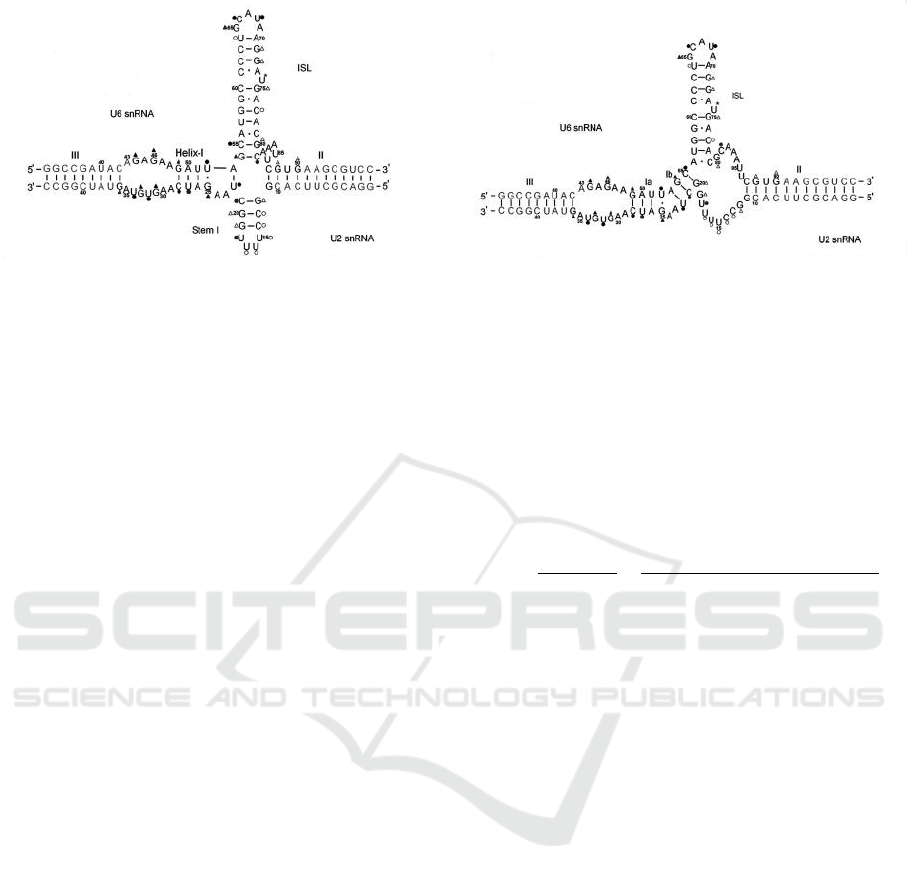
Figure 5: U2-U6 snRNA complex in humans obtained by Greenbaum’s lab (Zhao et al., 2013). The 4-way junction appears
on the left hand side with Helix I, and the 3-way junction appears on the right hand side with Helices Ia and Ib.
ergodicity (Durbin et al., 1998), the Gibbs guaran-
tee is that (S
t
1
,...,S
t
m
) for large t is a sample from
P(S
1
,...,S
m
), which is not necessarily a known distri-
bution, in contrast to P(S
l
|S
1
,...,S
l−1
,S
l+1
,...,S
m
)
which is reasonably accessible.
This is interesting because, conditioned on
S
1
,...,S
l−1
,S
l+1
,...,S
m
, the permissible windows of
the form w(l, i, j,u, v) are exactly those which do not
overlap with windows in S
l−1
and S
l+1
. As such, we
assume that (recall that we use w(l,i, j,u, v) to denote
both a window and its weight, depending on context):
P(S
l
|S
1
,...,S
l−1
,S
l+1
,...,S
m
) = P(S
l
|S
l−1
,S
l+1
)
P(S
l
|S
l−1
,S
l+1
) ∝
0 S
l
contains a window that
overlaps in S
l−1
or S
l+1
exp
h
∑
w(l,i, j,u,v)∈S
l
w(l,i, j,u,v)
i
otherwise
The exponential term is similar in spirit to the stan-
dard Boltzman distribution used for RNAs, knowing
that w(l,i, j,u,v) represents the negative of the en-
ergy.
If P(S
l
|S
l−1
,S
l+1
) is easy to sample from, then the
Gibbs sampler works nicely given a fixed mapping of
RNAs to levels 1 to m. Such mapping may be ob-
tained from the heuristic algorithm of Figure 2 (we
typically use 1/2, 1/3 or 1/4 for ε). We describe in
the next section how to sample from P(S
l
|S
l−1
,S
l+1
).
4.2 Gibbs Sampling with
Metropolis-Hastings
The Metropolis-Hastings algorithm for sampling
(also known as the Markov Chain Monte Carlo
method) was described in (Metropolis et al., 1953)
and (Hastings, 1970), and since then has been uti-
lized extensively in the literature. To sample from
P(S
l
|S
l−1
,S
l+1
), we first drop all the windows of the
form w(l,i, j,u,v) that overlap in S
l−1
or S
l+1
. We
only work with the remaining windows of the form
w(l,i, j, u,v). We then construct a random sequence
S
0
l
,S
1
l
,..., where S
t
l
is a set of non-overlapping win-
dows of the form w(l,i, j, u,v). This can be done with
a Metropolis-Hastings strategy: Given S
t
l
, we ran-
domly generate S
t+1
l
with some proposal probability
Q(S
t+1
l
|S
t
l
), and either accept S
t+1
l
with probability
min
n
1,
Q(S
t
l
|S
t+1
l
)
Q(S
t+1
l
|S
t
l
)
×
exp[
∑
w(l,i, j,u,v)∈S
t+1
l
w(l,i, j,u,v)]
exp[
∑
w(l,i, j,u,v)∈S
t
l
w(l,i, j,u,v)]
o
or reject it and let S
t+1
l
= S
t
l
.
It is well known and easy to show that such a
strategy results in a Markov chain which converges
to the desired probability distribution if the proposal
chain Q(S
t+1
l
|S
t
l
) satisfies Q(S
t+1
l
= y|S
t
l
= x) > 0 ⇔
Q(S
t+1
l
= x|S
t
l
= y) > 0; this also makes it irreducible
(Gallager, 2012).
For practical purposes, we limit S
t
l
to con-
tain only windows w(l, i, j,u,v) where u = v and
w(l,i, j, u,v) > 0. We also do not allow two adja-
cent windows w(l, i, j,u, v) and w(l, i − u, j − v, u
0
,v
0
)
to co-exists (since together they represent one bigger
window). With that in mind, a simple strategy is to
make Q(S
t+1
l
|S
t
l
) uniform among all the neighbors of
S
t
l
, where a neighbor can be obtained by one of the
following three operations:
• a window w(l,i, j,u, v) ∈ S
t
l
is removed from S
t
l
• a window w(l, i, j,u,v) 6∈ S
t
l
that does not overlap
in S
t
l
is added to S
t
l
• a window w(l,i, j,u,v) ∈ S
t
l
is replaced by a win-
dow w(l,i
0
, j
0
,u
0
,v
0
) 6∈ S
t
l
that only overlaps with
w(l,i, j, u,v) in S
t
l
Therefore, for every S
t+1
l
that is a neighbor of
S
t
l
, Q(S
t+1
l
|S
t
l
) is the inverse of the number of neigh-
bors of S
t
l
. This proposal probability defines an ir-
reducible Markov chain since every pair of solutions
A Sampling Approach for Multiple RNA Interaction - Finding Sub-optimal Solutions Fast
79

(a) candidate 1
I1 3’ UGUAUG
|||
U2 5’ ACAGAGAUGAUC--AGC
||||| |||
U6 3’ AUGA-UGUGAACUAGAUUCG
|||| ||||
I2 5’ UACUAACACC
(b) candidate 2
I1 3’ UGUAUG
U2 5’ ACAGAGAUGAUC--AGC
||||| |||
U6 3’ AUGA-UGUGAACUAGAUUCG
|||| ||||
I2 5’ UACUAACACC
(c) candidate 3
I1 3’ UGUAUG
|||
U2 5’ ACAGAGAUGAUCAGC
|||||
U6 3’ AUGA-UGUGAACUAGAUUCG
|||| ||||
I2 5’ UACUAACACC
(d) candidate (4)
I1 3’ UGUAUG
|||
U2 5’ ACAGAGAUGAUC--AGC
||||| |||
U6 3’ AUGAUGUGAACUAGAUUCG
||||
I2 5’ UACUAACACC
(e) candidate 5
I1 3’ UGUAUG
U2 5’ ACAGAGAUGAUCAGC
|||||
U6 3’ AUGA-UGUGAACUAGAUUCG
|||| ||||
I2 5’ UACUAACACC
(f) candidate 6
I1 3’ UGUAUG
U2 5’ ACAGAGA-UGAUC--AGC
|| ||||| |||
U6 3’ AUGAUGUGAACUAGAUUCG
||||
I2 5’ UACUAACACC
Figure 6: The yeast spliceosome with 4 RNAs (I1 and I2 are
functionally independent stretches of the same much longer
messenger RNA). (a) Helix Ia and helix Ib with both introns
attached. (b) Helix Ia and helix Ib with I1 detached. (c) He-
lix Ia with both introns attached. (d) Helix Ia and helix Ib
with I2 partially detached. (e) Helix Ia with I1 detached.
(f) Helix Ia and helix Ib with I1 detached and I2 partially
detached, moving towards detaching both introns, as would
happen when U2 and U6 are bound optimally in a full pari-
wise interaction.
can be reached from one another through a sequence
of neighbors.
4.3 A Distance Metric for Sub-optimal
Solutions
Many of the sampled sub-optimal solutions will be
similar. To quantify this similarity/dissimilarity, we
need a notion of a distance. We adopt an approach
inspired by the Jaccard metric (Jaccard, 1901).
To motivate this approach, we first define the no-
tion of a terminal window: Given a solution S, the
terminal window w(l,i, j,u, v) ∈ S is the window with
the largest l such that no windows appear on its right
in levels l − 1, l, and l + 1:
• no window w(l − 1,i
0
, j
0
,u
0
,v
0
) ∈ S has j
0
> i
(a) candidate 1
CopA 5’ CGGUUUAAGUGGG...UUUCGUACUCGCCAAAGUUGAAGA...UUUUGCUU 3’
||||||||||||| |||||||||||||||||||||||| ||||||||
CopT 3’ GCCAAAUUCACCC...AAAGCAUGAGCGGUUUCAACUUCU...AAAACGAA 5’
(b) candidate 2
CopA 5’ CGGUUUAAGUGGG...UUUCGUACUCGCCAAAGUUGAAGA...UUUUGCUU 3’
||||||||||||| ||||||||||||||||||||||||
CopT 3’ GCCAAAUUCACCC...AAAGCAUGAGCGGUUUCAACUUCU...AAAACGAA 5’
Figure 7: CopA-CopT in E. Coli. (a) The best solution
found. (b) A solution closer to the one observed in bio-
logical experiments in which the third interaction window
in non-existent.
• no window w(l,i
0
, j
0
,u
0
,v
0
) ∈ S has i
0
> i
• no window w(l + 1,i
0
, j
0
,u
0
,v
0
) ∈ S has i
0
> j
By recursively eliminating the terminal window from
a solution, we obtain a total order on the windows of
that solution. If two solutions are similar, we expect
them to have a similar set of windows; furthermore,
these windows should exhibit the same order.
In more detail, given a solution S, define
|S| as the number of windows in S, and let
w(l
1
,i
1
, j
1
,u
1
,v
1
),. ..,w(l
|S|
,i
|S|
, j
|S|
,u
|S|
,v
|S|
) be the
|S| windows in the order defined by terminal win-
dows. Each of these windows, say w(l,i, j,u,v), de-
fines the two intervals, [i − u + 1,i] in level l and
[ j −v +1, j] in level l +1. Define the set of interaction
intervals
I(S) = (I
1
,. .., I
2|S|
) = ([i
1
− u
1
+ 1,i
1
],[ j
1
− v
1
+ 1, j
1
],. ..
.. .,[i
|S|
− u
|S|
+ 1,i
|S|
],[ j
|S|
− v
|S|
+ 1, j
|S|
])
as an ordered sequence of 2|S| intervals, and L(S) =
(l
1
,...,l
|S|
) as an ordered sequence of |S| levels,
where l
i
is the level defining the i
th
window. There-
fore, L(S) means that we have the following set of
pairwise interactions (not necessarily unique in terms
of RNAs): RNA l
1
with RNA l
1
+ 1, RNA l
2
with
RNA l
2
+ 1, . .., RNA l
|S|
with RNA l
|S|
+ 1. Two
solutions that do not agree on this set, are consid-
ered completely dissimilar; otherwise, their distance
is given by the amount of overlap in their interaction
intervals (as in the Jaccard metric), hence the follow-
ing definition of distance:
Given two solutions S
1
with I(S
1
) = (I
1
,I
2
,...)
and S
2
with I(S
2
) = (T
1
,T
2
,...), the distance between
S
1
and S
2
is
d(S
1
,S
2
) =
(
1 L(S
1
) 6= L(S
2
)
1 −
∑
i
|I
i
∩T
i
|
∑
i
|I
i
∪T
i
|
L(S
1
) = L(S
2
)
where ∩ and ∪ represent the standard intersection and
union operations on sets respectively, and intervals
are treated as sets of integers. This distance is a metric
in [0,1] (Mneimneh and Ahmed, 2015).
BIOINFORMATICS 2016 - 7th International Conference on Bioinformatics Models, Methods and Algorithms
80

4.4 Clustering the Samples
The sampled sub-optimal solutions are generally
more than what we need. In addition, as mentioned
above, many of them will be similar. Therefore,
we use clustering to reduce their number. To clus-
ter the samples, we first remove duplicates, so we
only work with unique samples. We adopt hierar-
chical agglomerative clustering with single linkage
and the silhouette index (Rousseeuw, 1987) to deter-
mine the optimal number of clusters. Given a solu-
tion S, let c(S) be its cluster. Let b
j
(S) be the average
distance from S to all solutions in cluster j, and let
b(S) = min
j6=c(S)
b
j
(S). We assume that the number
of clusters is at least 2, so b(S) is defined. Let a(S)
be the average distance from S to all other solutions
in c(S). If S is a singleton in its cluster, we make
a(S) = b(S). The silhouette of a solution S is given
by
b(S) − a(S)
max[a(S),b(S)]
and is always in the interval [−1, 1]. A silhouette
close to 1 means that solution S is well situated in its
cluster since a(S) b(S). The silhouette of a clus-
ter is the average silhouette of all the solutions in the
cluster. The silhouette index is the average of all the
cluster silhouettes. We seek the number of clusters
that maximizes this index. The beauty of this index
follows from that it is always bounded, works for ar-
bitrary notions of distance (dissimilarity), and does
not require the use of a cluster centroid, which is typ-
ically not trivial to find for non-Euclidean distances.
Given a number of clusters, the optimal solu-
tion in each cluster acts as a “representative” of the
cluster. The representatives should reveal some of
the structures that are observed in biological experi-
ments (Ahmed and Mneimneh, 2014; Mneimneh and
Ahmed, 2015).
5 EXPERIMENTAL RESULTS
We allow 100 iterations for the “burn-in” time of the
Metropolis-Hastings algorithm to obtain the first sam-
ple, and 50 iterations between consecutive samples
thereafter. We note that we can generate a 1000 so-
lutions (Gibbs samples) in just a few seconds, which
is several orders of magnitude improvement over the
previous exhaustive approach in (Ahmed and Mneim-
neh, 2014; Mneimneh and Ahmed, 2015).
After clustering, we sort the representatives of the
clusters by decreasing weight. Then to assess our ap-
proach, for each experiment we have a number k of
candidate structures in mind; for instance, Figure 6
shows six candidates (k = 6), and Figure 7 shows two
candidates (k = 2). Given that set of candidates, we
only consider the first ≤ k representatives, but we still
record the total number of clusters obtained. For each
candidate S, and using the distance metric described
earlier, we find the representative R that is closest to
S. If S = R, that’s a direct hit (a distance of zero).
Otherwise, if among the k candidates, the closest to
R is S itself, we declare this as a “close” hit with the
given distance. In this case, and after converting the
windows of S and R to bonds, we also compute their
F1-score (Powers, 2011) given by:
F1-score = 2 ×
precision × recall
precision + recall
where precision is defined as the number of bonds in
R that are also in S divided by the number of bonds in
R, and recall is defined as the number of bonds in R
that are also in S divided by the number of bonds in S.
If there are no direct or close hits for candidate S, we
declare a miss.
We repeat the experiment 100 times and compute
the average number of unique samples and the aver-
age number of clusters obtained, and for each of the k
candidates, the percentage of direct hits, the average
distance and average F1-score of close hits, and the
percentage of misses.
5.1 Experiment 1: Structural Variation
The U2-U6 complex in the spliceosome of yeast has
been reported to have two distinct experimental struc-
tures, e.g. (Sashital et al., 2004). In one conformation,
U2 and U6 interact to form a helix known as helix
Ia. In another conformation, the interaction reveals a
structure containing an additional helix, known as he-
lix Ib. Section 3 describes possible underlying mech-
anisms that are responsible for this conformational
switch. We consider the set of six candidates in Fig-
ure 6. Tables 1 and 2 summarize the results of this
experiment using 1000 samples for k = 4 and k = 6
respectively, supporting the fact that the two confor-
mations show up. With 1000 samples, the first k can-
didates always show up with a 100% hit.
5.2 Experiment 2: Artifact Interactions
Due to the optimization nature of the problem, it is
sometimes easy to pick up interactions that are not
biologically real. This is because dropping these in-
teractions from the solution would make it less opti-
mal (even when preferred biologically, as described
in Section 3). The third interaction window of CopA-
CopT in Figure 7 is an example of such an artifact.
A Sampling Approach for Multiple RNA Interaction - Finding Sub-optimal Solutions Fast
81

Table 1: Yeast spliceosome. 100 runs, 100 samples in each
run, avg. number of unique samples: 70.82, avg. number of
clusters: 11.07, k = 6.
candidate %hit avg. distance avg. F1-score %miss
1 98 0.1 0.947 0
2 90 0.118 0.938 1
3 69 0.106 0.944 3
4 68 0.106 0.937 13
5 52 0.123 0.934 13
6 44 0.079 0.959 47
Table 2: Yeast spliceosome. 100 runs, 100 samples in each
run, avg. number of unique samples: 70.82, avg. number of
clusters: 11.07, k = 4.
candidate %hit avg. distance avg. F1-score %miss
1 98 0.1 0.947 0
2 90 0.118 0.938 1
3 69 0.118 0.937 17
4 68 0.067 0.966 30
5 30 0.121 0.936 67
6 7 - - 93
For the two candidates of Figure 7 (k = 2), Tables 3
and 4 summarize the results of this experiment using
100 and 1000 samples respectively, showing that we
succeed in dropping the undesired window.
Table 3: CopA-CopT. 100 runs, 100 samples in each run,
avg. number of unique samples: 72.26, avg. number of
clusters: 2.55, k = 2.
candidate %hit avg. distance avg. F1-score %miss
1 39 0.082 0.980 0
2 2 0.094 0.950 60
Table 4: CopA-CopT. 100 runs, 1000 samples in each run,
avg. number of unique samples: 505.1, avg. number of
clusters: 2.37, k = 2.
candidate %hit avg. distance avg. F1-score %miss
1 99 0.022 0.989 0
2 30 0.052 0.973 3
6 CONCLUSION
In multiple RNA interaction, the best structure may
not be the real structure, and the real structure may
not be unique. In this work, we build on a previous
approach (exhaustive enumeration) to generate multi-
ple sub-optimal solutions using the Pegs and Rubber
Bands formulation. Here, an approach using Gibbs
sampling and the Metropolis-Hastings algorithm is
developed, and provides a much faster alternative to
exhaustive enumeration.
This new sampling approach successfully com-
putes sub-optimal solutions for the multiple RNA in-
teraction problem that are truthful representations of
the actual biological structures. For instance, it can
provide several candidate structures when they exist,
e.g. the U2-U6 complex and its introns in the spliceo-
some of yeast, and find structures that agree with the
literature, but are not necessarily optimal in the com-
putational sense, e.g. CopA-CopT in E. Coli.
REFERENCES
Ahmed, S. A. and Mneimneh, S. (2014). Multiple rna inter-
action with sub-optimal solutions. In Bioinformatics
Research and Applications, pages 149–162. Springer.
Ahmed, S. A., Mneimneh, S., and Greenbaum, N. L.
(2013a). A combinatorial approach for multiple
rna interaction: Formulations, approximations, and
heuristics. In Computing and Combinatorics, pages
421–433. Springer.
Ahmed, S. A., Mneimneh, S., and Greenbaum, N. L.
(2013b). A combinatorial approach for multiple
rna interaction: Formulations, approximations, and
heuristics. In Computing and Combinatorics, pages
421–433. Springer Berlin Heidelberg.
Alkan, C., Karakoc, E., Nadeau, J. H., Sahinalp, S. C., and
Zhang, K. (2006). Rna-rna interaction prediction and
antisense rna target search. Journal of Computational
Biology, 13(2):267–282.
Andronescu, M., Zhang, Z. C., and Condon, A. (2005).
Secondary structure prediction of interacting rna
molecules. Journal of molecular biology, 345(5):987–
1001.
Cao, S. and Chen, S.-J. (2006). Free energy landscapes of
rna/rna complexes: with applications to snrna com-
plexes in spliceosomes. Journal of molecular biology,
357(1):292–312.
Chen, H.-L., Condon, A., and Jabbari, H. (2009). An o(n
5
)
algorithm for mfe prediction of kissing hairpins and
4-chains in nucleic acids. Journal of Computational
Biology, 16(6):803–815.
Chitsaz, H., Backofen, R., and Sahinalp, S. C. (2009a).
birna: Fast rna-rna binding sites prediction. In Algo-
rithms in Bioinformatics, pages 25–36. Springer.
Chitsaz, H., Salari, R., Sahinalp, S. C., and Backofen, R.
(2009b). A partition function algorithm for interact-
ing nucleic acid strands. Bioinformatics, 25(12):i365–
i373.
Ding, Y. and Lawrence, C. E. (2003). A statistical sampling
algorithm for rna secondary structure prediction. Nu-
cleic acids research, 31(24):7280–7301.
Dirks, R. M., Bois, J. S., Schaeffer, J. M., Winfree, E., and
Pierce, N. A. (2007). Thermodynamic analysis of in-
teracting nucleic acid strands. SIAM review, 49(1):65–
88.
Durbin, R., Eddy, S. R., Krogh, A., and Mitchison, G.
(1998). Biological sequence analysis: probabilis-
tic models of proteins and nucleic acids, Chapter 11.
Cambridge university press.
BIOINFORMATICS 2016 - 7th International Conference on Bioinformatics Models, Methods and Algorithms
82

Gallager, R. G. (2012). Discrete stochastic processes,
Chapter 4, volume 321. Springer Science & Business
Media.
Geman, S. and Geman, D. (1984). Stochastic relaxation,
gibbs distributions, and the bayesian restoration of
images. Pattern Analysis and Machine Intelligence,
IEEE Transactions on, (6):721–741.
Hastings, W. K. (1970). Monte carlo sampling methods us-
ing markov chains and their applications. Biometrika,
57(1):97–109.
Huang, F. W., Qin, J., Reidys, C. M., and Stadler, P. F.
(2009). Partition function and base pairing probabili-
ties for rna–rna interaction prediction. Bioinformatics,
25(20):2646–2654.
Jaccard, P. (1901). Etude comparative de la distribution
florale dans une portion des Alpes et du Jura. Impr.
Corbaz.
Kolb, F. A., Engdahl, H. M., Slagter-J
¨
ager, J. G., Ehres-
mann, B., Ehresmann, C., Westhof, E., Wagner, E.
G. H., and Romby, P. (2000a). Progression of a loop–
loop complex to a four-way junction is crucial for the
activity of a regulatory antisense rna. The EMBO jour-
nal, 19(21):5905–5915.
Kolb, F. A., Malmgren, C., Westhof, E., Ehresmann, C.,
Ehresmann, B., Wagner, E., and Romby, P. (2000b).
An unusual structure formed by antisense-target rna
binding involves an extended kissing complex with
a four-way junction and a side-by-side helical align-
ment. Rna, 6(3):311–324.
Li, A. X., Marz, M., Qin, J., and Reidys, C. M. (2011). Rna–
rna interaction prediction based on multiple sequence
alignments. Bioinformatics, 27(4):456–463.
Liu, J. S. (1994). The collapsed gibbs sampler in bayesian
computations with applications to a gene regulation
problem. Journal of the American Statistical Associa-
tion, 89(427):958–966.
McCaskill, J. S. (1990). The equilibrium partition function
and base pair binding probabilities for rna secondary
structure. Biopolymers, 29(6-7):1105–1119.
Metropolis, N., Rosenbluth, A. W., Rosenbluth, M. N.,
Teller, A. H., and Teller, E. (1953). Equation of state
calculations by fast computing machines. The journal
of chemical physics, 21(6):1087–1092.
Metzler, D. and Nebel, M. E. (2008). Predicting rna sec-
ondary structures with pseudoknots by mcmc sam-
pling. Journal of mathematical biology, 56(1-2):161–
181.
Meyer, I. M. (2008). Predicting novel rna–rna interactions.
Current opinion in structural biology, 18(3):387–393.
Mneimneh, S. (2009). On the approximation of optimal
structures for rna-rna interaction. IEEE/ACM Trans-
actions on Computational Biology and Bioinformatics
(TCBB), 6(4):682–688.
Mneimneh, S. and Ahmed, S. A. (2015). Multiple rna inter-
action: Beyond two. To appear in IEEE Transactions
on NanoBioscience.
Mneimneh, S., Ahmed, S. A., and Greenbaum, N. L.
(2013). Multiple RNA interaction - formulations, ap-
proximations, and heuristics. In BIOINFORMATICS
2013 - Proceedings of the International Conference
on Bioinformatics Models, Methods and Algorithms,
Barcelona, Spain, 11 - 14 February, 2013., pages 242–
249.
M
¨
uckstein, U., Tafer, H., Hackerm
¨
uller, J., Bernhart, S. H.,
Stadler, P. F., and Hofacker, I. L. (2006). Ther-
modynamics of rna–rna binding. Bioinformatics,
22(10):1177–1182.
Newby, M. I. and Greenbaum, N. L. (2001). A conserved
pseudouridine modification in eukaryotic u2 snrna in-
duces a change in branch-site architecture. RNA,
7(06):833–845.
Pervouchine, D. D. (2004). Iris: intermolecular rna interac-
tion search. Genome Informatics Series, 15(2):92.
Powers, D. M. (2011). Evaluation: from precision, recall
and f-measure to roc, informedness, markedness and
correlation.
Rousseeuw, P. J. (1987). Silhouettes: a graphical aid to
the interpretation and validation of cluster analysis.
Journal of computational and applied mathematics,
20:53–65.
Salari, R., Backofen, R., and Sahinalp, S. C. (2010). Fast
prediction of rna-rna interaction. Algorithms for
molecular Biology, 5(5).
Sashital, D. G., Cornilescu, G., and Butcher, S. E. (2004).
U2–u6 rna folding reveals a group ii intron-like do-
main and a four-helix junction. Nature structural &
molecular biology, 11(12):1237–1242.
Sun, J.-S. and Manley, J. L. (1995). A novel u2-u6 snrna
structure is necessary for mammalian mrna splicing.
Genes & Development, 9(7):843–854.
Tong, W., Goebel, R., Liu, T., and Lin, G. (2013). Ap-
proximation algorithms for the maximum multiple rna
interaction problem. In Combinatorial Optimization
and Applications, pages 49–59. Springer.
Tong, W., Goebel, R., Liu, T., and Lin, G. (2014). Approx-
imating the maximum multiple rna interaction prob-
lem. Theoretical Computer Science.
Wei, D., Alpert, L. V., and Lawrence, C. E. (2011). Rnag:
a new gibbs sampler for predicting rna secondary
structure for unaligned sequences. Bioinformatics,
27(18):2486–2493.
Zhao, C., Bachu, R., Popovi
´
c, M., Devany, M., Brenowitz,
M., Schlatterer, J. C., and Greenbaum, N. L. (2013).
Conformational heterogeneity of the protein-free hu-
man spliceosomal u2-u6 snrna complex. RNA,
19(4):561–573.
A Sampling Approach for Multiple RNA Interaction - Finding Sub-optimal Solutions Fast
83

APPENDIX
RNA Sequences
CopA-CopT in E. Coli.
CopA (even)
5’ CGGUUUAAGUGGGCCCCGGUAAUCUUUUCGUACUCGCCA
AAGUUGAAGAAGAUUAUCGGGGUUUUUGCUU 3’
CopT (odd)
5’ AAGCAAAAACCCCGAUAAUCUUCUUCAACUUUGGCGAGU
ACGAAAAGAUUACCGGGGCCCACUUAAACCG 3’
Human Spliceosome
I1 (odd)
5’ NNNNNNNNNNGUAUGUNNNNNNNNNN 3’
U6 (even)
5’ AUACAGAGAAGAUUAGCAUGGCCCCUGCGCAAGGAUGAC
ACGCAAAUUCGUGAAGCGU 3’
U2 (odd)
5’ ACGCUUCACGGCCUUUUGGCUAAGAUCAAGUGUAGUAU 3’
I2 (even)
5’ NNNNNNNNNNUACUAACNNNNNNNNNN 3’
Yeast Spliceosome
I1 (odd)
5’ NNNNGUAUGUNNNN 3’
U6 (even)
5’ ACAGAGAUGAUCAGC 3’
U2 (odd)
5’ GCUUAGAUCAAGUGUAGUA 3’
I2 (even)
5’ NNNNUACUAACACCNNNN 3’
BIOINFORMATICS 2016 - 7th International Conference on Bioinformatics Models, Methods and Algorithms
84
