A Mass-ﬂow based MILP Formulation for the Inventory Routing with

Explicit Energy Consumption

Yun He

1,2

, Cyril Briand

1,2

and Nicolas Jozefowiez

1,3

CNRS, LAAS, 7 Avenue du Colonel Roche, F-31400 Toulouse, France

Univ. de Toulouse, UPS, LAAS, F-31400 Toulouse, France

Univ. de Toulouse, INSA, LAAS, F-31400 Toulouse, France

Keywords:

Inventory Routing Problem, Energy Minimization, Mixed Integer Linear Programming.

Abstract:

In this paper, we present a new mass-ﬂow based Mixed Integer Linear Programming (MILP) formulation for

the Inventory Routing Problem (IRP) with explicit energy consumption. The problem is based on a multi-

period single-vehicle IRP with one depot and several customers. Instead of minimizing the distance or inven-

tory cost, the problem takes energy minimization as an objective. In this formulation, ﬂow variables describing

the transported mass serve as a link between the inventory control and the energy estimation. Based on phys-

ical laws of motion, a new energy estimation model is proposed using parameters like vehicle speed, average

acceleration rate and number of stops. The solution process contains two phases with different objectives: one

with inventory and transportation cost minimization as in traditional IRP, the other with energy minimization.

Using benchmark instances for inventory routing with parameters for energy estimation, experiments have

been conducted. Finally, the results of these two solution phases are compared to analyse the inﬂuence of

energy consumption to the inventory routing systems.

1 INTRODUCTION

Our purpose is to introduce an energy estimation

method and to propose a MILP optimization model

that incorporates energy consumption into the Inven-

tory Routing Problem (IRP) with mass ﬂows. We start

from a general literature review of the IRPs and the

emerging Green Vehicle Routing Problems (GVRPs),

then we discuss the incorporation of these two prob-

lems to present our new formulation.

The Vendor Managed Inventory (VMI) is an in-

ventory management model where the supplier mon-

itors the inventory level of the whole system and

acts as a central decision maker for the long-term

replenishment policy of each retailer. With respect

to the traditional Retailer Managed Inventory (RMI),

the VMI results in a more efﬁcient resource utiliza-

tion (Archetti et al., 2007). Under the context of

the VMI, the IRP combines the inventory manage-

ment, vehicle routing and scheduling. There are three

simultaneous decisions to make (Coelho et al., 2013):

1. when to serve a customer;

2. how much to deliver when serving a customer;

3. how to route the vehicle among the customers to

be served.

The IRP was ﬁrst studied under the context of

the distribution of industrial gases (Bell et al., 1983).

After that, numbers of variants of the problem have

come out, but there exists no standard version. The

trade-offs between inventory costs and transportation

costs are studied and explicit formulas to evaluate

these trade-offs based on spatial density of customers

are obtained in (Burns et al., 1985). In (Dror and Ball,

1987), the authors proposed a method to reduce the

long-term version of the problem to a single-period

problem by deﬁning single-period costs that reﬂects

long-term effects. In (Anily and Federgruen, 1990),

the authors tried to decide the long-run replenish-

ment strategies for a set of geographically dispersed

retailers and they proposed the ﬁrst clustering algo-

rithm for the IRP. In (Savelsbergh and Song, 2007),

the authors studied the inventory routing with con-

tinuous moves with both pick-ups and deliveries and

developed a randomized greedy algorithm. The in-

ventory routing with backlogging is studied in (Ab-

delmaguid et al., 2009), where a heterogeneous ﬂeet

is considered. In (Archetti et al., 2007), the authors

242

He, Y., Briand, C. and Jozefowiez, N.

A Mass-ﬂow based MILP Formulation for the Inventory Routing with Explicit Energy Consumption.

DOI: 10.5220/0005698802420251

In Proceedings of 5th the International Conference on Operations Research and Enterprise Systems (ICORES 2016), pages 242-251

ISBN: 978-989-758-171-7

proposed a MILP formulation of the IRP and applied

a Branch-and-Cut algorithm to solve this problem.

Later in (Archetti et al., 2014), based on the formu-

lation in the previous paper, new formulations are de-

veloped and compared with existing formulations us-

ing a large set of benchmark instances.

Two important literature reviews are worth men-

tioning here. (Andersson et al., 2010) is a survey

of the industrial aspects of the problem, and (Coelho

et al., 2013) is a comprehensive review on the typolo-

gies of the problem as well as their solution methods.

Nowadays, the Supply Chain Management is

faced with a new challenge—the sustainability. As

one of the three bottom lines of Sustainable Sup-

ply Chain Management, environmental sustainability

is the most recognized dimension (Fish, 2015). As

shown in (Sahin et al., 2009), energy costs account

for about 60% of the total cost of a unit of cargo trans-

ported on road.

In the literature, there are a growing number of pa-

pers about the green logistics and sustainable supply

chain management. However, most of them treat the

inventory management and the vehicle routing sepa-

rately. The Energy Minimizing Vehicle Routing Prob-

lem (EMVRP) is studied in (Kara et al., 2007), where

the Capacitated Vehicle Routing Problem (CVRP) is

extended with a new cost function based on distance

and load of the vehicle. In (Xiao et al., 2012), a Fuel

Consumption Rate (FCR) considered CVRP is pro-

posed to minimize the fuel consumption. Focusing on

the pollution and CO

emission generated by the road

transport sector, the Pollution Routing Problem (PRP)

is proposed to explicitly control the Greenhouse Gas

(GHG) emission of the transportation (Bektas¸ and La-

porte, 2011). The only paper that incorporates envi-

ronmental aspects in the IRP is a case study from the

petrochemical industry and total CO

emissions are

considered as a cost in the objective function (Treitl

et al., 2014).

A detailed literature review of the GVRP can be

found in (Lin et al., 2014). In this review, the environ-

mental sensitive Vehicle Routing Problem is divided

into three groups: the Green-VRP for the optimiza-

tion of energy consumption; the PRP for the reduction

of pollution, especially GHG emissions; and the Ve-

hicle Routing in Reverse Logistics for the wastes and

end-of-life product collection. The authors point out

that incorporating inventory models with PRP models

can be promising.

This brief survey indicates that there lacks en-

ergy awareness in the inventory routing, or there lacks

a system wide view in the sustainable routing. As

the IRP integrates several decisions for the inventory

control of the whole system, it helps us to make strate-

gic decisions for energy optimization. First, under

the VMI policy, the customer demands are ﬂexible

and can be distributed in different combinations. This

property allows us to determine an optimal set of de-

livery quantities that yields the most environmental

cost effectiveness while making sure that stock-out

never happens. Second, the order of visit and the ve-

hicle routes are to be determined. It is thus possible

to design a routing strategy that takes the roads with

the least energy costs. Third, the time of visit is also

adaptable. We can choose a delivery time that is both

convenient for the customers and that can also avoid

rush hours, as congestion is one of the causes of high

energy consumption and CO

emissions.

Our study focuses on the integration of the IRP

with explicit consideration on the energy consump-

tion in the transportation. The main contributions of

this paper are: (i) to propose an approach to estimate

the energy consumed in the transportation activities

of inventory routing; (ii) to reformulate the IRP to ex-

plicitly incorporate the energy consideration; (iii) to

analyse the possible energy savings and the trade-offs

between energy savings, travelled distances and in-

ventory costs.

The remainder of this paper is organized as fol-

lows: in Section 2, the problem is described in de-

tails. Then, the mathematical model is presented in

Section 3. After that, experimentation and results are

given in Section 4, followed by the conclusion in Sec-

tion 5.

2 PROBLEM STATEMENT

The problem in our study is based on a multi-period

single-vehicle deterministic inventory routing prob-

lem with one depot and several customers. The vehi-

cle can leave the depot only once per period. In each

period, it makes a tour around the customers that need

to be reﬁlled and returns to the depot. Stock-out and

back-orders are not allowed in the model. Instead of

the distance and inventory minimization, we take en-

ergy minimization as objective. Both the Maximum

Level (ML) and the Order-up-to Level (OU) policy

are applied to see the inﬂuence of different replenish-

ment strategies to the energy consumption. A detailed

explanation of these policies is given in Section 3.

To facilitate the energy estimation, two units are

used to measure inventory components—the number

of components and the weight in kilograms (kg). The

number of components is used by the customers to

represent their inventory levels and to count the num-

ber of packages of delivered goods. The weight is

used by the transporters. It is the physical mass of the

A Mass-ﬂow based MILP Formulation for the Inventory Routing with Explicit Energy Consumption

243

components transported by the vehicle.

The next parts present in details the parameters

and variables of the problem and the computation of

the energy estimation function. In particular, mass

ﬂow variables are introduced to link energy estima-

tion and inventory management.

2.1 General Settings for Routing

The problem is constructed on a complete undirected

graph G = {V,E}. V = {0,.. .,n} is the vertex set. It

includes one depot denoted by 0 and the customers to

visit denoted by the set V

= {1, ...,n}. E = {(i, j) |

i, j ∈ V and i < j} is the set of undirected edges.

There are T replenishment planning periods. Each

period can be a day, a week or even a month accord-

ing to the real situation. In each period, only one tour

can be performed. If a tour is presented in a period,

the vehicle starts from the depot, travels through all

the customers who need to be served at this period

and returns back to the depot at the end of the period.

Three kinds of decision variables z

, x

i j

and y

i j

correspond to routing. For each i ∈ V

, t ∈ T , z

is a bi-

nary variable indicating whether customer i is served

at period t. It equals 1 if customer i is served and 0

otherwise. Particularly, z

indicates whether the tour

at period t is performed (equals 1) or not (0). For

each edge (i, j) ∈ E and each period t ∈ T , x

i j

is an

integer variable indicating the number of times that

edge (i, j) is used in the tour of period t. For each arc

(i, j) ∈ V ×V and each period t ∈ T , variable y

i j

is a

binary variable to indicate the direction of the vehicle

route. It equals 1 if the vehicle travels from node i to

j at period t and 0 otherwise.

The vehicle has a capacity Q expressed in num-

bers of components and a mass limit M. The empty

vehicle mass, or curb weight (kg) of the vehicle is W .

2.2 Inventory Characteristics

Inventory levels at customers and depot are monitored

during the whole planning time horizon. They are

summarised at the end of each replenishment period.

The customer demands are described as demand rates

per period. In each period, r

units of components are

demanded by customer i ∈ V

. In particular, r

is the

number of components made available at the depot

in each period. Each customer i ∈ V

has a stocking

capacity C

while the depot is supposed to have an un-

limited stocking capacity. h

is the inventory storage

cost per unit of component per period at customer i or

the depot. The weight of a component in kilograms at

customer i ∈ V

is denoted by m

Two variables are deﬁned for the inventory man-

agement. The variable I

is the inventory level in num-

ber of components at the depot 0 or at the customer

i ∈ V

at the end of period t. The variable q

is the

number of components delivered to customer i ∈ V

during period t ∈ T .

2.3 Energy Estimation

There are many complicated models in the literature

that estimate the CO

emissions or the amount of pol-

lutants produced by a vehicle on road. (Demir et al.,

2014) is a review of vehicle emission models and

their inclusion into the existing optimization methods.

However, few models focus on the energy consumed

and most of them depend on vehicle type. This can

be partly explained by the fact that the main power

source of vehicles used today is petroleum. Neverthe-

less, with the emergence of electric and hybrid vehi-

cles, we ﬁnd it more appropriate to estimate the en-

ergy consumption instead of fuel consumption. In

addition, for the generality of the problem, it is im-

portant that the model would apply for every type of

vehicles. According to (Samaras and Ntziachristos,

1998), travelling kinematic variation (accelerations,

idle duration, etc.) obviously affects engine load and

by turns the energy consumption. Thus, in this paper,

we propose a general simple model based on vehicle

dynamics. This model would be applicable to Euro-

pean suburban transportation network with short or

medium distances and potentially high trafﬁc inten-

sity. It can give us a gross estimation of the energy re-

quired by a vehicle on a road segment with speed vari-

ation, independent of vehicle type or energy source.

In our model, the stop rate τ, i.e., the number of

stops per unit of distance is used to model the dy-

namics of the vehicle on a ﬁxed segment of road.

This parameter can also represent the trafﬁc condi-

tion on the road. More precisely, with a trafﬁc near

free ﬂow, τ takes a value near 0, which means that

the vehicle goes through the road ﬂuently without any

stops; however, with congestion, this number is set

to a bigger value to indicate a frequent speed varia-

tion. Usually τ takes a value between 0 and 4 de-

pending on road types (Andr

e et al., 1998). Moreover,

there exists an interrelationship between the distance

travelled, the stop rate and the speed and acceleration

of the vehicle, which is generally explained in Sec-

tion 4.1 and is not the subject of our study.

Suppose a vehicle travelling from one location to

another. The path of the vehicle between two loca-

tions is supposed to be predeﬁned with an average

stop rate τ, and the total distance travelled is s. So the

vehicle stops τ·s times during the trip. The coefﬁcient

ICORES 2016 - 5th International Conference on Operations Research and Enterprise Systems

244

Target speed

acceleration

uniform

deceleration

time

velocity

stop

. . .

Figure 1: The speed variation of the vehicle with time.

of friction is a ﬁxed parameter µ = 0.01. The gravita-

tional acceleration is g = 9.81m/s

. The environmen-

tal effects of the road (wind, temperature etc.) as well

as the viscosity of air are ignored. Road slopes are

also ignored for the moment but will be considered in

the future. As a result, the only forces exerted on the

vehicle are the rolling resistance and the traction.

Between every two stops, the vehicle speed is

supposed to follow a ﬁxed pattern of variation—

acceleration, uniform speed movement and stop (Fig-

ure 1). Each time, the vehicle speeds up from 0 to

the target speed V with a ﬁxed acceleration a

acc

. It

goes on at this speed for a while and then stops. The

stop is supposed to be instantaneous. This pattern is

repeated τ · s times supposing that the vehicle has no

speed at both the starting and the ending point. After

each stop, it speeds up again to the same target speed.

The next part explains how to estimate energy

consumption using this simple model.

The mathematical relationship between the physi-

cal quantities of energy (E), work (W ) and power (P)

are:

E =

P(t)dt

P(t) = Fv(t)

E = W =

∑

with F a constant force, v(t) the speed at instant t and

s the distance travelled.

According to knowledge of physics and energy

conservation, under the hypothesis of speed variation

presented above, the total energy cost per unit of mass

when distance s is travelled with stop rate τ is then:

c = gµs + τsV

(1)

Figure 2 shows the power variation of the vehicle un-

der the previous speed variation. We can see that each

time the vehicle speeds up, there appears a ”peak” of

engine power which corresponds to a potentially high

energy consumption. This is also reﬂected by Equa-

tion 1—the more the vehicle stops on a road segment

(τ takes a bigger value), the higher the energy would

cost. See the Appendix for the detailed calculation.

In this way, we deﬁne c

i j

= gµs

i j

+ τ

i j

the

energy cost per unit of mass for each edge (i, j). It is

acceleration

uniform

deceleration

time

power

stop

. . .

Figure 2: The power variation with time.

related to the distance travelled s

i j

and the dynamics

of the vehicle on the road as expressed by the stop rate

i j

and target speed V

i j

If m

i j

(kg) of mass is loaded on the vehicle when

traversing from i to j and the vehicle weighs W (kg),

the energy cost of the vehicle travelling from i to j is

thus:

i j

+W ) (2)

2.4 Commodity Mass Flow

As we can see from the energy estimation computa-

tion, the total energy cost is a linear function of mass.

Meanwhile, the mass or the quantity of products is

also an important element in the inventory manage-

ment. It is a measurement of the inventory levels. In

fact, there exists a mass ﬂow inside the transportation

network and it can serve as a bridge linking the inven-

tory routing and the energy optimization.

In the traditional IRP formulations presented

in (Archetti et al., 2014), a ﬂow formulation exists

to model the inventory ﬂows inside the transportation

network. Our model takes advantage of this formula-

tion. Instead of considering the ﬂow in terms of num-

ber of components, the mass of the shipped compo-

nents is considered. Once we decide the mass trans-

ported on each edge of the network at each period,

we can deduce the number of components left at each

customer vertex. Or inversely, if we know how many

units of components are delivered to each customer

at each period, we can decide the order of visits and

get a ﬂow of mass in the transportation network that

minimizes the energy consumed.

In our model, variables m

i j

are deﬁned as the mass

transported by the vehicle from i to j at period t. They

are linked with the vehicle ﬂow variables y

i j

. If the

vehicle does not go from i to j at period t (y

i j

= 0),

i j

is equal to 0.

Figure 3 details the various ﬂows traversing cus-

tomer i at period t. The inventory ﬂow I

and the

demand r

, expressed in number of components, are

associated with the dotted arcs. They describe the

variation of the inventory level of i with time periods.

The solid arcs stand for the mass of the incoming and

A Mass-ﬂow based MILP Formulation for the Inventory Routing with Explicit Energy Consumption

245

j∈V \{i}

i, t

j∈V \{i}

t−1

Figure 3: The ﬂows passing through customer i at period t.

outgoing products (m

and m

i j

respectively). They

are used to estimate the potential energy consumption,

with c

i j

the energy cost per unit of mass on edge (i, j).

The difference

(

∑

j∈V\{i}

−

∑

j∈V\{i}

i j

) gives the

number of components q

delivered by the vehicle to

customer i during period t.

3 MATHEMATICAL MODEL

In this section, we present the mathematical model

using the mass ﬂow.

3.1 Objectives

Two objectives are deﬁned, one for inventory and dis-

tance optimization and the other for energy optimiza-

tion. The objective function (3) is the traditional one

as in (Archetti et al., 2014). It is the sum of the total

distance travelled plus the sum of the inventory stor-

age costs over all the periods.

min

∑

t∈T

∑

(i, j)∈V ×V

i j

∑

t∈T

∑

i∈V

(3)

The objective function (4) is the sum of the total en-

ergy consumed in the inventory routing over all the

periods. Note that it contains two terms: one is a ﬂex-

ible cost related to the transported mass of the vehicle

i j

, and the other is a ﬁxed cost induced by the vehi-

cle curb weight W .

min

∑

t∈T

∑

(i, j)∈V ×V

i j

∑

t∈T

∑

(i, j)∈V ×V

i j

(4)

3.2 Constraints

Here are the sets of constraints. Compared with the

basic ﬂow formulation in (Archetti et al., 2014), mass

ﬂow variables take place of commodity ﬂow vari-

ables.

Inventory Management

Constraints (5) to (9) are for monitoring the inventory

levels of each location at each period.

= I

t−1

+ r

−

∑

i∈V

∀t ∈ T (5)

= I

t−1

− r

+ q

∀i ∈ V

,t ∈ T (6)

≥ C

− I

t−1

∀i ∈ V

,t ∈ T (7)

≤ C

− I

t−1

∀i ∈ V

,t ∈ T (8)

≤ C

∀i ∈ V

,t ∈ T (9)

Constraints (5) and (6) ensure that the inventory lev-

els of each station are coherent from one period to

another. The OU inventory policy is ensured by con-

straints (7) and (8)—after each delivery, the inventory

level of each visited customer is fulﬁlled to the max-

imum. If we delete Constraints (7), the model be-

comes one under the ML policy, where the replen-

ishment level is ﬂexible but bounded by the stocking

capacity of each customer. Constraints (9) ensure that

if a customer i is not visited at a period t (z

= 0), the

delivered quantity q

equals 0 and if the customer is

visited, the delivered quantity never exceeds the ca-

pacity.

Commodity Mass Flow Management

Constraints (10) and (11) are the mass ﬂow con-

straints.

∑

j∈V

0 j

∑

i∈V

∀t ∈ T (10)

∑

j∈V

−

∑

j∈V

i j

= q

∀i ∈ V

,t ∈ T (11)

Constraints (10) ensure that at period t, the mass out

of the depot is equal to the total mass transported to all

the customers. Constraints (11) ensure that for each

customer i at each period t, the quantity received is

equal to the difference between the entering and the

leaving mass ﬂow.

Vehicle Routing

Constraints (12) to Constraints (17) are typical

routing constraints.

Undirected Routing

∑

j∈V

0 j

= 2z

∀t ∈ T (12)

∑

j∈V

j<i

∑

j∈V

j>i

i j

= 2z

∀i ∈ V

,t ∈ T (13)

ICORES 2016 - 5th International Conference on Operations Research and Enterprise Systems

246

Directed Vehicle Flow

∑

j∈V

0 j

= z

∀t ∈ T (14)

∑

j∈V

i j

= z

∀t ∈ T,i ∈ V

(15)

∑

j∈V

= z

∀t ∈ T,i ∈ V

(16)

i j

= y

i j

+ y

∀t ∈ T,(i, j) ∈ E (17)

Constraints (12) and (13) deﬁne the non-directed

route of the vehicle in each period. Constraints (14)–

(16) restrain the direction of the vehicle ﬂow. They

link y and z variables to make sure that in each period

at most one tour is performed and that each customer

is visited at most once in each period. Constraints (17)

link variables y and x to ensure that each edge is used

at most once in each period.

Vehicle Capacity

Constraints (18) and (19) guarantee that the vehicle

capacity is never exceeded both in number of compo-

nents and in unit of mass.

∑

i∈V

≤ Qz

∀t ∈ T (18)

i j

≤ My

i j

∀t ∈ T,(i, j) ∈ V ×V (19)

Constraints (19) also link the mass ﬂow and the vehi-

cle ﬂow on the graph. They make sure that the direc-

tion of the vehicle ﬂow is the same as that of the mass

ﬂow.

Variable Domains

Constraints (20)–(26) are the variable domains.

0 ≤ I

≤ C

∈ N ∀i ∈ V,t ∈ T (20)

0 ≤ q

≤ Q,q

∈ N ∀i ∈ V

,t ∈ T (21)

0 ≤ m

i j

≤ M, m

i j

∈ N ∀(i, j) ∈ V ×V,t ∈ T (22)

∈ {0,1} ∀i ∈ V,t ∈ T (23)

i j

∈ {0,1} ∀(i, j) ∈ E,i < j,t ∈ T (24)

0 j

∈ {0,1,2} ∀ j ∈ V

,t ∈ T (25)

i j

∈ {0,1} ∀(i, j) ∈ V ×V,t ∈ T (26)

All the variables take integer values. Note that for

variables x

0 j

, since direct routing is possible, they can

be assigned with value 2.

3.3 Solution Methodology

The solution process is divided into two phases. In the

ﬁrst phase, the objective is to minimize the combined

cost of transportation and inventory as in objective

function (3). In the second phase, starting with the

solution of the ﬁrst phase, the same model is solved to

minimize the total energy consumption as computed

in objective function (4).

The methodology allows us to quickly ﬁnd a feasi-

ble solution for energy minimization in the ﬁrst phase,

and then explore the energy minimization possibilities

in the second phase.

4 EXPERIMENTATION

This section explains the data generation method,

gives the system settings and provides an analysis of

the obtained results.

4.1 Data Generation

Based on existing IRP instances proposed in (Archetti

et al., 2007), new instances more adapted to energy

estimation are generated. Information on stop rates τ

and vehicle target speeds V relative to the distance

is added in the existing instances. The correlation

within these parameters is determined based on em-

pirical data of delivery trucks on real routes provided

by (Walkowicz et al., 2014). The following part ex-

plains how the data set is generated.

First, three types of road is considered—highway,

national route and urban road. For each edge between

two locations, the type of road is generated randomly.

Then, target speed and number of stops for different

types of roads are generated using different methods.

Details of these methods are given in the Appendix.

Finally, for all types of road, the average acceleration

is ﬁxed at 1.01m/s

Then, a random number between 1 and 10 is gen-

erated for each customer i to represent the mass of a

package of components m

. Vehicle weight and mass

capacity are correlated according to vehicle informa-

tion provided in (EcoTransIT World Initiative (EWI),

2014).

In total, 256 cases are generated. Each case con-

tains 5 instances. The cases are categorized by the

number of periods (3 or 6 periods of replenishment

planning), the proportion of the inventory storage cost

in relation to the transportation cost (high or low), the

inventory replenishment policy (OU or ML), the pro-

portion of each type of road in the whole map and the

number of customers in the map.

4.2 System Settings

The model is realized in C++ with IBM



ILOG



CPLEX 12.6.1.0 and solved by the default Branch-

and-Bound algorithm with one thread. The operation

A Mass-ﬂow based MILP Formulation for the Inventory Routing with Explicit Energy Consumption

247

system is Ubuntu 14.04 LTS with Intel



Core



i7-

4790 3.60GHz processor and 16 G memory.

A time limit of 1800 seconds is set for each of

the two phases. All the other settings of CPLEX are

as default. The results of both of the two phases are

compared in the next part.

4.3 Result Analysis

Performance

Eventually, within the time limit, nearly 70% of the

instances with distance and inventory optimization

can be solved to optimality by CPLEX, while only

one third of the instances can be solved to optimality

with energy minimization. Table 1 gives a summary

of the performance information.

The dimension of the instance is determined by

the number of periods (”T” column in the table) and

the number of customers (”n” column in the table).

The inventory policy (OU or ML) changes the con-

straint sets of the model. A combination of these three

parameters deﬁne a category of instances. Each cate-

gory contains 40 instances. In this table, computation

time of each solution phase (”time1” and ”time2”)

and the solution status within the time limit (”status1”

and ”status2”) are presented. The times are average

values over all the instances of the same category. If

all the instances of this category can be solved to opti-

mality by CPLEX, the status is noted ”Optimal”. Oth-

erwise, the average relative gap after 1800 seconds of

computation is reported.

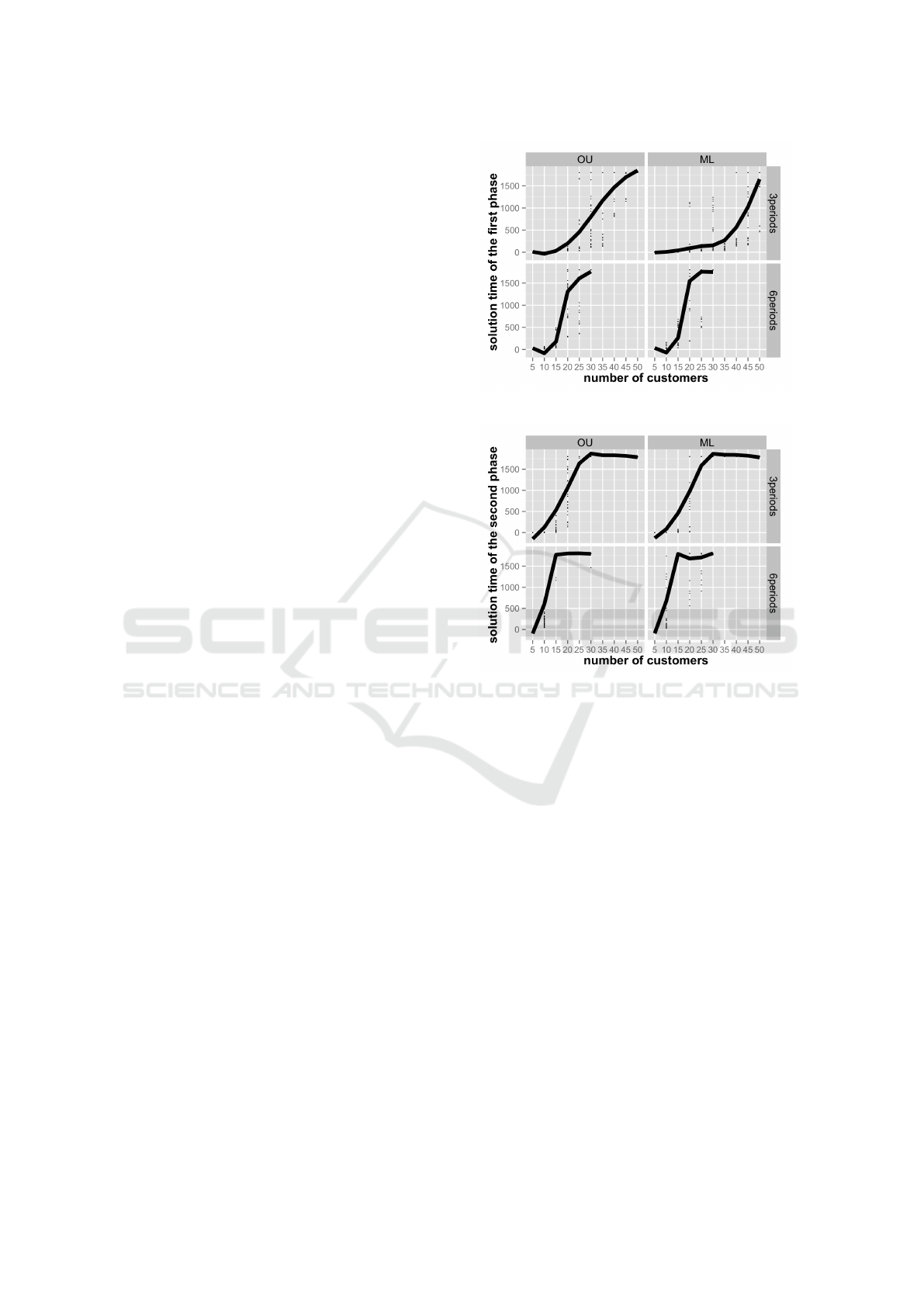
As we can see from this table, energy minimiza-

tion is much more difﬁcult to solve than inventory and

transportation cost minimization (time2  time1).

This may result from the large possible combination

of the values of the mass ﬂows. It is normal to see that

the problem becomes more difﬁcult as the dimension

of the instances increases. For both OU and ML poli-

cies, instances larger than 20 customers with 3 periods

or 15 customers with 6 periods become impossible

to solve for energy optimization (Phase 2) within the

time limit. And it seems that the inﬂuence of the in-

ventory policy to energy minimization is not as much

as in the traditional IRP. Figure 4 and 5 show the solv-

ing time increase with the number of customers for

different number of periods and inventory policies.

Energy Reduction

In general, 95 % of all the instances can expect an en-

ergy reduction. Of all the instances where energy is

reduced, the average reduction is 3.7%, and the max-

imum reduction can reach 19.4%. Meanwhile, the

distance and inventory cost remains nearly the same

Figure 4: Solution time of the ﬁrst phase.

Figure 5: Solution time of the second phase.

(with an average augmentation rate of less than 1%).

In addition, the experiments show that nearly all of the

instances with 6 periods can be assigned an energy-

saving replenishment strategy and nearly 90% of the

instances with 3 periods can achieve a solution with

less energy consumption.

By inspecting the results in details, it is observed

that most of the energy reduction comes from the

transported mass, which correspond to the ﬂexible

part of the energy minimizing objective function. The

energy reduction induced by the transported mass is

nearly 20% in average and it can reach as high as

66.3%. And by analysing the energy objective func-

tion, it is easy to see that minimizing the ﬁxed part of

the energy cost or the part induced by the curb weight

is equivalent to a weighted minimization of the dis-

tance. Since the vehicle mass accounts for nearly half

of the total mass moving on the road, a great part of

the energy minimization is equivalent to distance min-

imization. This can explain the reason why ﬁnally the

total energy reduction is so small even though the en-

ergy consumed by transporting the products can be

highly reduced.

ICORES 2016 - 5th International Conference on Operations Research and Enterprise Systems

248

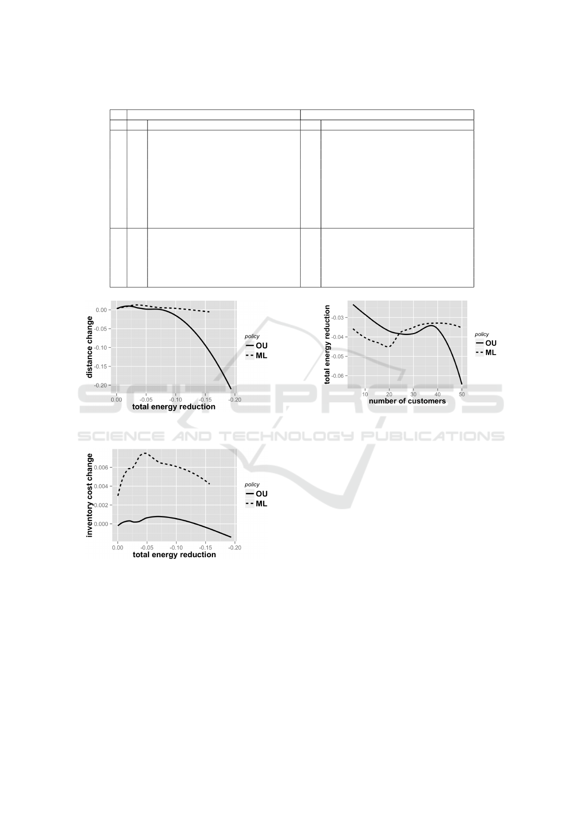
Table 1: Performance summary of all the instances.

OU policy ML Policy

T n time1 time2 status1 status2 n time1 time2 status1 status2

5 0.0665 0.108 Optimal Optimal 5 0.142 0.0759 Optimal Optimal

10 1.84 3.44 Optimal Optimal 10 2.37 2.47 Optimal Optimal

15 14.9 83.8 Optimal Optimal 15 10.0 23.6 Optimal Optimal

20 53.6 1235.4 Optimal 0.0228 20 138.8 1075.9 Optimal 0.0645

25 642.7 1799.1 0.0114 0.0594 25 71.33 1800.0 Optimal 0.1053

30 721.9 1800.0 0.0106 0.1028 30 307.1 1800.0 Optimal 0.1175

35 1079.4 1800.0 0.0196 0.132 35 112.6 1800.0 Optimal 0.1362

40 1624.6 1800.0 0.0336 0.1679 40 570.4 1800.0 0.0380 0.1564

45 1729.6 1800.0 0.0572 0.2185 45 1043.3 1800.0 0.0233 0.1873

50 1800.0 1799.6 0.0767 0.2260 50 1645.8 1800.0 0.0175 0.2108

5 0.694 1.194 Optimal Optimal 5 4.021 1.243 Optimal Optimal

10 26.94 234.7 Optimal Optimal 10 45.39 324.6 Optimal 0.0201

15 177.2 1769.9 Optimal 0.0342 15 262.1 1789.8 Optimal 0.0465

20 1307.7 1800.0 0.0372 0.1133 20 1545.3 1679.6 0.0180 0.1115

25 1449.7 1800.0 0.0298 0.1349 25 1563.9 1720.7 0.0304 0.1501

30 1800.0 1791.6 0.0453 0.1792 30 1800.0 1800.0 0.0416 0.1748

Figure 6: The relationship between distance and energy re-

duction.

Figure 7: The relationship between inventory and energy

reduction.

It should also be noted that the inventory policy

has an inﬂuence on the energy minimization poten-

tial. Figure 6 and 7 show the relationship between

distance (inventory) and energy reduction. The solid

curves represent average values of all the instances.

We can see that under the OU policy, most of the re-

duction is obtained by minimizing the distance trav-

elled. The more energy reduction there is, the less dis-

tance would be travelled. Under the ML policy, most

of the reduction is obtained by changing the inven-

Figure 8: The relationship between energy reduction and

number of customers under different inventory policy.

tory replenishment strategy. This could result from

the fact that the ML policy is more ﬂexible than the

OU policy.

Figure 8 shows the energy reduction in relation

to the number of customers under different policies.

We can see that for small instances, ML policy tends

to produce a lower cost, but with the increase of the

dimension of instances, the model becomes more dif-

ﬁcult to solve with ML policy than with OU policy,

so for the most difﬁcult instances where non-optimal

solution is reached within the time limit, it is still OU

policy that gives a better result. These results imply

that inventory replenishment strategy is important for

energy minimization. Instead of always ﬁll the inven-

tory to the maximum level as suggested by OU policy,

ML policy may give a better energy solution.

We could not observe much relationship between

road types and energy minimization. In fact, the in-

ﬂuence of road types to the energy reduction becomes

noticeable only for instances with large number of

customers. This could result from a lack of realis-

tic data. So more tests should be done with more

realistic datasets. And the solution method should

be improved so that realistic-sized instances could be

A Mass-ﬂow based MILP Formulation for the Inventory Routing with Explicit Energy Consumption

249

solved to optimality to show the energy saving poten-

tial of different road types.

5 CONCLUSIONS

Energy consumption is an important aspect in both

economical and ecological view. It becomes more

and more important with the sustainable requirement

of the inventory systems. However, few researchers

paid attention to the combination of inventory man-

agement, vehicle routing and energy minimization.

This new mass ﬂow-based formulation of the IRP

with energy consumption addresses the problem ex-

plicitly. An energy estimation method is proposed

that combines vehicle dynamics and road character-

istics. This estimation gives us an energy cost func-

tion that is linear to the total mass. In this new IRP

formulation, the mass is added as a decision variable

and the energy cost function is considered as an objec-

tive. The relationship between the vehicle dynamics

in the transportation network, the inventory manage-

ment strategy and the energy consumption estimation

is examined. Our ﬁrst experimentation shows that a

better energy cost can be achieved by adjusting the

inventory replenishment planning. Among all the in-

ﬂuence factors, the inventory policy is an important

one.

Further works need to be done on the modelling

of trafﬁc networks, so that different road types, espe-

cially road slops, trafﬁc conditions as well as vehi-

cle speed levels could be considered in the decision

process. The estimation of the energy costs needs to

be more representative. More data are needed from

the real world to accomplish the work. The inventory

routing model needs to be improved to better control

the time and quantity of each delivery. Solution al-

gorithms and heuristics are to be explored to speed

up the computation, especially with realistic data that

would contain larger number of customers or longer

decision periods. The extension of the problem to a

multi-objective one is also a promising track of study.

ACKNOWLEDGEMENTS

This work was supported by the ECO-INNOVERA-

1rst call EASY (ANR-12-INOV-0002).

REFERENCES

Abdelmaguid, T. F., Dessouky, M. M., and nez, F. O.

(2009). Heuristic approaches for the inventory-routing

problem with backlogging. Computers and Industrial

Engineering, 56(4):1519–1534.

Andersson, H., Hoff, A., Christiansen, M., Hasle, G., and

Lø kketangen, A. (2010). Industrial aspects and

literature survey: Combined inventory management

and routing. Computers and Operations Research,

37(9):1515–1536.

Andr

e, M., Hassel, D., and Weber, F.-j. (1998). Devel-

opment of short driving cycles–Short driving cycles

for the inspection of in-use cars –Representative Eu-

ropean driving cycles for the assessment of the I/M

schemes. Technical Report May, INRETS - LEN,

Laboratoire

Energie Nuisances.

Anily, S. and Federgruen, A. (1990). One Warehouse Mul-

tiple Retailer Systems with Vehicle Routing Costs.

Management Science, 36(1):92–114.

Archetti, C., Bertazzi, L., Laporte, G., and Grazia Sper-

anza, M. (2007). A Branch-and-Cut Algorithm for a

Vendor-Managed Inventory-Routing Problem. Trans-

portation Science, 41(3):382–391.

Archetti, C., Bianchessi, N., Irnich, S., and Grazia Sper-

anza, M. (2014). Formulations for an inventory rout-

ing problem. International Transactions in Opera-

tional Research, 21:353–374.

Bektas¸, T. and Laporte, G. (2011). The pollution-routing

problem. 45:1232–1250.

Bell, W. J., Dalberton, L. M., Fisher, M. L., Greenﬁeld,

A. J., Jaikumar, R., Kedia, P., Mack, R. G., and Prutz-

man, P. J. (1983). Improving the Distribution of Indus-

trial Gases with and On-Line Computerized Routing

and Scheduling Optimizer. Interfaces, 13(6):4–23.

Burns, L. D., Hall, R. W., Blumenfeld, D. E., and Daganzo,

C. F. (1985). Distribution Strategies that Minimize

Transportation and Inventory Costs.

Coelho, L. C., Cordeau, J.-F., and Laporte, G. (2013).

Thirty Years of Inventory Routing. Transportation

Science, 48(1):1–19.

Demir, E., Bektas¸, T., and Laporte, G. (2014). A review of

recent research on green road freight transportation.

European Journal of Operational Research, 237:775–

793.

Dror, M. and Ball, M. (1987). Inventory/routing: Reduc-

tion from an annual to a short-period problem. Naval

Research Logistics (NRL), 34:891–905.

EcoTransIT World Initiative (EWI) (2014). Ecological

Transport Information Tool for Worldwide Transports

Methodology and Data—Update .

Fish, L. A. (2015). Applications of Contemporary Manage-

ment Approaches in Supply Chains.

Kara, I., Kara, B. Y., and Yetis, M. K. (2007). Energy Min-

imizing Vehicle Routing Problem. Verlag Berlin Hei-

delberg, 1:62–71.

Lin, C., Choy, K. L., Ho, G. T. S., Chung, S. H., and Lam,

H. Y. (2014). Survey of Green Vehicle Routing Prob-

lem: Past and future trends. Expert Systems with Ap-

plications, 41:1118–1138.

Sahin, B., Yilmaz, H., Ust, Y., Guneri, A. F., and Gulsun,

B. (2009). An approach for analysing transportation

costs and a case study. European Journal of Opera-

tional Research, 193(1):1–11.

ICORES 2016 - 5th International Conference on Operations Research and Enterprise Systems

250

Samaras, Z. and Ntziachristos, L. (1998). Average hot emis-

sion factors for passenger cars and light duty trucks.

Technical Report LAT report No. 9811, Lab. of Ap-

plied Thermodynamics, Aristotle University of Thes-

saloniki.

Savelsbergh, M. and Song, J. H. (2007). Inventory routing

with continuous moves. Computers and Operations

Research, 34:1744–1763.

Treitl, S., Nolz, P. C., and Jammernegg, W. (2014). Incor-

porating environmental aspects in an inventory rout-

ing problem. A case study from the petrochemical in-

dustry. Flexible Services and Manufacturing Journal,

26:143–169.

Walkowicz, K., Duran, A., and Burton, E. (2014). Fleet dna

project data summary report. Technical report, NREL.

Xiao, Y., Zhao, Q., Kaku, I., and Xu, Y. (2012). Devel-

opment of a fuel consumption optimization model for

the capacitated vehicle routing problem. Computers

and Operations Research, 39(7):1419–1431.

APPENDIX

Energy Estimation

According to knowledge of physics and energy con-

servation, under the hypothesis of speed variation pre-

sented in Section 2.3, we have:

• In each acceleration phase, the speed of the ve-

hicle increases from 0 to the target speed V with

constant acceleration a

acc

. With F

acc

the traction

force of the engine, s

acc

the distance travelled,

acc

the energy consumed, and P

acc

(t) the engine

power:

v(t) = a

acc

(t) =

acc

− mgµ = ma

acc

(t) = F

acc

v(t) = m(a

acc

+ gµ)a

acc

− mgµs

acc

At the end of this phase, the engine power is

acc

= m(a

acc

+ gµ)V

the distance travelled is

acc

The total energy cost per unit of mass is

acc

= gµs

acc

• In the uniform-speed phase, the distance s

computed as the difference between the total dis-

tance s and the total distance travelled in acceler-

ation and deceleration. Since the deceleration is

considered to be instantaneous (s

dec

= 0), the total

distance travelled at uniform speed is calculated

as:

= s − τ s (s

acc

+ s

dec

) = s − τ s s

acc

with τ · s the total number of stops. The engine

power is also constant

(t) = F

V = mgµV

The total energy cost per unit of mass in the uni-

form phase is:

= gµ(s − τ s s

acc

• In each deceleration phase, since we consider an

instantaneous stop,

dec

= 0

dec

(t) = 0

dec

and the energy cost per unit of mass is

dec

the total energy cost per unit of mass when distance s

is travelled with stop rate τ is then:

c = c

+ τ · s (c

acc

+ c

dec

Finally, we get:

c = gµs + τsV

Calculation of Parameters for Different

Road Types

On a highway, the maximum speed is ﬁxed at

110km/h, and the number of stops is ﬁxed at 2 stops

per edge independent of the road distance travelled.

On a national route, the vehicle speed is ﬁxed at

80km/h and the number of stops is linearly depen-

dent on the distance with a random error. On an ur-

ban road, both the stop rate and the vehicle speed are

dependent on the distance travelled. The stop rate τ

is determined by a linear function of the distance as

in the case of national route. And the target speed V

is derived from the stop rate τ by an equation of the

form V = β + α

· τ + α

/τ.

A Mass-ﬂow based MILP Formulation for the Inventory Routing with Explicit Energy Consumption

251