
Unsupervised Clustering of Hyperspectral Images of Brain Tissues by
Hierarchical Non-negative Matrix Factorization
Bangalore Ravi Kiran
1
, Bogdan Stanciulescu
1
and Jesus Angulo
2
1
Centre de Robotique(CAOR), MINES ParisTech, PSL-Research University, Paris, France
2
Centre de Morphologie Mathematique(CMM), MINES ParisTech, PSL-Research University, Fontainebleau, France
Keywords:
Hyperspectral Image, Unsupervised Clustering, Brain Tissue, Non-negative Matrix Factorization.
Abstract:
Hyperspectral images of high spatial and spectral resolutions are employed to perform the challenging task of
brain tissue characterization and subsequent segmentation for visualization of in-vivo images. Each pixel is
high-dimensional spectrum. Working on the hypothesis of pure-pixels on account of high spectral resolution,
we perform unsupervised clustering by hierarchical non-negative matrix factorization to identify the pure-
pixel spectral signatures of blood, brain tissues, tumor and other materials. This subspace clustering was
further used to train a random forest for subsequent classification of test set images constituent of in-vivo and
ex-vivo images. Unsupervised hierarchical clustering helps visualize tissue structure in in-vivo test images
and provides a inter-operative tool for surgeons. Furthermore the study also provide a preliminary study of the
classification and sources of errors in the classification process.
1 INTRODUCTION
Medical Hyperspectral imaging (MHSI) is a non-
invasive and non-ionizing modality used in robust tis-
sue identification, characterization achieved reason-
able classification and localization accuracy in of var-
ious kinds of cancerous tissues on account of vast
improvements in spectral and spatial imaging reso-
lutions (Lu and Fei, 2014). Discriminating cancer-
ous and normal tissues with Near Infra-Red (NIR)
spectroscopy has been an active topic in the past
two decades. (Panasyuk et al., 2007) study the use
of MHSI for identifying residual tumor in a resec-
tion bed and to indicate regions requiring more re-
section. (Lu et al., 2014) use HSI in-vivo to achieve
tumor identification in tumor bearing mice. (Liu
et al., 2011) study localization of tumor tissue on
the tongue of human patients using a tunable HSI
camera. In this study we study the characteriza-
tion and identification of brain tissues by perform-
ing joint clustering and un-mixing. We also demon-
strate the utility of the hierarchical clustering as a vi-
sual aid for inter-operative(IoP) procedures (Schulder
and Carmel, 2003) in the resection of cancerous tis-
sue. Though one should note that the standard in IoP
brain tumor surgery modality has been MRI, it is pre-
cise but a costly technology. Hyperspectral images
are cheaper and furthermore faster to acquire.
The primary goal of this paper is to address the
common problem of lack of an exact ground truth la-
bels in the hyperspectral images in-vivo. This pro-
duces a challenging problem of hyperspectral image
segmentation and classification. Our solution consists
in generating unsupervised clustering that can serve
as a stable identification and labeling, for a subse-
quent semi-supervised classification. Further we note
that, it is unrealistic to obtain a well localized marker
of tumors, in-vivo, during a surgical procedure, in
view of different constraints of space and time. Fi-
nally we also do not know the exact spectrum of can-
cerous and normal tissue at this stage of our study. We
do note that from previous studies on different tumor
types, normal and cancerous tissue spectra are close
(see subsection 4), and are difficult to distinguish.
We thus characterize the tissue by clustering their
spectrum in similar subspaces. This helps visualize
different structures in the tissue as well as locate tu-
mors and related structures. Unsupervised clustering
is rarely followed, for such problems, but given that
we operate at high spatial and spectral resolutions, we
stand to gain some useful information. We use the
clustering of ex-vivo tumors with surrounding tissue,
blood and other structures as a target model we pre-
dict the location of tumors in in-vivo images. Finally,
the clustering will also be used as tool by surgeons
and pathology to label the tissues to generate ground
Kiran, B., Stanciulescu, B. and Angulo, J.
Unsupervised Clustering of Hyperspectral Images of Brain Tissues by Hierarchical Non-negative Matrix Factorization.
DOI: 10.5220/0005697600770084
In Proceedings of the 9th International Joint Conference on Biomedical Engineering Systems and Technologies (BIOSTEC 2016) - Volume 2: BIOIMAGING, pages 77-84
ISBN: 978-989-758-170-0
Copyright
c
2016 by SCITEPRESS – Science and Technology Publications, Lda. All rights reserved
77
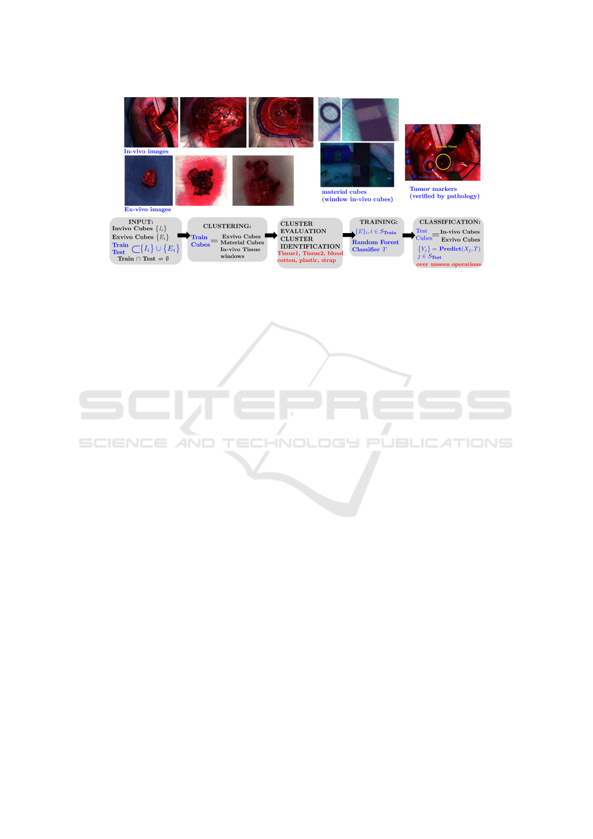
Figure 1: We classify the input images into three categories: In-vivo images (during surgery), Ex-vivo images (extracted tumor
after surgery) and material cubes (carefully windowed regions containing only surgical material). Black plastic rings markers
highlight the locations of healthy tissue and a tumor tissue in a scene. The ex-vivo images serve as localized target that ensure
the presence of tumor tissue in a localized window. We partition the operations into a training and test set, after which we
perform hierarchical clustering on the test images. The H2NMF clustering algorithm also performs unmixing and calculates
the endmembers for each cluster. We use clusters at a particular level to train a random forest classifier. We demonstrate the
classification on other ex-vivo and in-vivo images in the test set. The flow-diagram at the bottom illustrates all the steps in our
study.
truth data.
The primary contributions of the paper include the
identification of pure-spectrum or pure-pixels of ma-
terials using VNIR camera images of brain tumors by
applying the hierarchical clustering by 2-rank NMF
approximation (Gillis et al., 2015). Pure-pixels are
found at the leaves of this hierarchical structure and
correspond to rank-1 matrices. This is discussed in
section 2. We use the unsupervised clustering as su-
pervised labels to identify these pure-pixels in the
in-vivo images by training a decision forest. See
figure 1 for a summary of the work-flow. The or-
ganization of the paper is as follows. We describe
briefly the imaging setup in this section, in section
2 we provide a brief introduction to endmember ex-
traction, the separable non-negative matrix factoriza-
tion(NMF) and the hierarchical NMF decomposition
algorithm (Gillis et al., 2015) employed in this study.
Imaging Setup: The medical imaging demon-
strator consists of two camera pairs covering differ-
ent parts of the spectrum at different spatial reso-
lutions, a VNIR (visible-to-near-infrared) and NIR
(near-infrared cameras) cameras. The VNIR cam-
era captures 826 spectral bands, in the spectral range
of 400-1000 nm with a spectral resolution of 2-3
nm, and each pixel has a dimension of 0.1287 mm
x 0.1287 mm. While the NIR camera captures 172
spectral bands, in the spectral range of 900-1700 nm,
each pixel has a dimension of 0.48 mm x 0.48 mm.
We shall work with the VNIR camera images mainly
since they consist of precise spectral information. The
increment in wavelength is 1.9285 nm for the current
setup. Images are calibrated using a standard white
and dark reference.
In this study we work on hyperspectral images
from a VNIR camera with a very high spatial and
spectral resolution. Images were obtained of the brain
tissue and brain tumors, in-vivo (brain tissue open
during surgery) and ex-vivo (extracted brain tumor on
surgical table). Images were obtained over 20 opera-
tions. The images from both cameras were obtained
during the surgical procedure. The information of the
type of tumor and other associated patient information
was missing during the current paper’s study. This
will be discussed more in detail. The images were
taken during the surgical procedure (in-vivo) and right
after the procedure outside the body (ex-vivo) with
the extracted tumor placed under the camera. In this
paper we restrict our study to the VNIR camera im-
ages due to their high spectral and spatial resolution.
2 UNMIXING
Hyperspectral unmixing is the problem of inferring
which are the materials in the scene (visible directly
or visible as a mixture) by the general process of di-
mensionality reduction. This basically consists in de-
composing a hyperspectral image X = [x
1
, x
2
, ...x
n
]
with n pixels, where each pixel x
i
is p-dimensional
spectrum. The two elements of the decomposition
BIOIMAGING 2016 - 3rd International Conference on Bioimaging
78
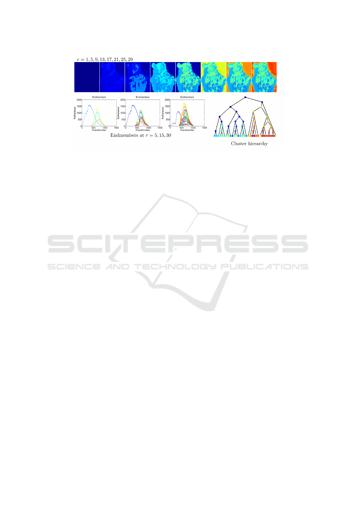
Figure 2: Segmentation Hierarchy showing a tumor ex-vivo decomposed at different levels r = 1 to 32 of the hierarchical
2-rank decomposition (H2NMF) algorithm. The 2-rank approximation divisional step is used is to arrive with a unit rank
matrices and the leaves of the hierarchical decomposition. The labels in the segmentations are consistently colored to match
with the tree nodes. They help show the persistence of a subspace/clustering visually. This tree structure gives an visual idea of
the structure of the tissue, labels in that are close in terms subspaces branch. By viewing the endmembers (spectra) at different
levels, we can infer visually that blood is a dominant material in the scene (blue peak around 400nm). The shallow clusters
correspond to submatrices of low approximation error which close to rank-1 and thus correspond to a single tissue/material.
are a set of r reference spectra or endmembers and
W = [w
1
, w
2
, ...w
r
] and their relative proportions at
each pixel(abundances) H = [h
1
, h
2
, ...h
n
], where, w
i
is a p-dimensional spectrum and h
i
is r-dimensional
coefficient weights. The spectrum at a pixel is a con-
vex composition of endmembers. This imposes two
conditions: Firstly the abundances need to be positive
and the sum of abundances by each endmember sum
to unity at each pixel (Ma et al., 2014). The goal of
the hyperspectral unmixing(HU) or endmember ex-
traction process is to obtain the spectrum that corre-
sponds to “pure” materials in the scene. This can be
a complex problem based on the physical interactions
between the materials, rays and the reflections. We
assume the Linear mixing model(LMM) for its inher-
ent simplicity and popularity in the remote sensing
community. The model assumes that at a given pixel
location the incident ray interacts only with one mate-
rial in the true site of the pixel. Given the spectral and
spatial resolution of the VNIR camera, this assump-
tion seems to be a reasonable.
Separable NMF: Endmember extraction is well stud-
ied as a problem of non-negative matrix factoriza-
tion problem since it respects the endmember con-
straints. It is written as a matrix factorization problem
X ≈ W H, where this approximation is often evaluated
by minimizing the Frobenius norm of the residual
kX −WHk
2
F
. Independent of how the decomposition
is calculated the NMF, geometrically it generates the
vectors h
i
(endmembers) whose simplicial cone con-
tains all the data points {x
i
} ∈ X. There can be many
cones possible and the decomposition is non-unique.
In case of high spatial and spectral resolution of HSI
cubes, one can make the hypothesis that there exists
pixels in the image which themselves form the bound-
ing vertices of the a convex cone, and thus directly
the endmembers. Physically this means that given a
pixel spectrum we can infer the material it contains
and be sure that its contribution is from a single ma-
terial. This is called the separability condition (Gillis
and Luce, 2014) under which we obtain a unique and
tractable decomposition of the NMF problem. Geo-
metrically, the separability condition reformulates the
NMF problem as that of finding the extreme rays of
the conical hull of a finite set of vectors. Given a HSI
cube X ∈ R
n×p
, we can write its separable NMF de-
composition as
X = W H = W [I
r
, H
0
]Π (1)
where W ∈ R
m×r
, H
0
> 0, Π is a permutation matrix,
which rotates the r different endmembers. Columns
of W are the endmembers, while the entry H(i, j) are
the abundances/scalar coefficient of the ith endmem-
ber at the jth pixel in X. Geometrically this corre-
sponds to the convex hull of the columns of X.
Hierarchical Two-rank NMF: The hierarchical two
rank NMF (H2NMF) first introduced in the paper
(Gillis et al., 2015) aims at obtaining a rank-1 sub-
matrix by hierarchical application of a NMF decom-
position. The decomposition step consists of a, first
projecting the data points on to the first two eigen
vectors, and thus a 2-d cone, by calculating the singu-
lar value decomposition(SVD). Second, the direction
matrix is approximated by a separable NMF decom-
positions, namely the SPA (Gillis and Luce, 2014) of
the data points under decomposition.
This yields pure-pixels in the HSI cube approxi-
mating the first principle component. The goal is to
Unsupervised Clustering of Hyperspectral Images of Brain Tissues by Hierarchical Non-negative Matrix Factorization
79

finally arrive with a set of leaves which which are of
rank. This corresponds to pure-pixel or a single ma-
terial. Though this hierarchical method is provided,
the stopping condition for the growth of the hierarchy
is not provided. Instead this is a parameter of the al-
gorithm that determines the number of endmembers
being extracted. At each step of this divisional hier-
archical clustering step, the approximation error min-
imized is (Gillis et al., 2015),
E
k
= σ
2
1
(X(:, K
1
i
))+σ
2
1
(X(:, K
2
i
))−σ
2
1
(X(:, K
i
)) (2)
where σ
1
refers to the first singular value of the ma-
trices, and K
i
corresponds to the indices of the parent
and K
1
i
, K
2
i
are indices of the child clusters in the bi-
nary split. This approximation error corresponds to
the rank approximation of input cluster or matrix.
The split is decided by choosing line after the pro-
jection on to a 2-d cone. This is chosen by parameter
δ
∗
(see algorithm 1) so as to have a balanced set of
points across the split (Gillis et al., 2015) as well a
clusters with elements that are homogeneous.
The H2NMF algorithm apart from clustering per-
forms unmixing by generating and endmember asso-
ciated with each cluster. To evaluate the endmem-
ber corresponding to a cluster that is supposed to be
a rank-1 approximation of sub-matrices, we follow
(Gillis et al., 2015)’s measure. Mean removed spec-
tral angle(MRSA) is defined for any two pairs of spec-
tra x, y as:
φ(x, y) =
1
π
arccos
(x − ¯x)
T
(y − ¯y)
kx − ¯xk
2
ky − ¯yk
2
∈ [0, 1] (3)
where for a vector z ∈ R
m
, ¯z =
∑
m
i=1
z
i
. The MRSA
provides the a measure to compare the pure-pixel
in the input sub-matrix and its endmember spectrum
produced by a rank-2 NMF decomposition. We use
MRSA to evaluate the homogeneity of the hierarchi-
cal clustering at different levels.
We use the H2NMF algorithm (see Algo. 1) to
provide a hierarchical subspace decomposition of the
ex-vivo cubes to recover the pure-pixels by varying
the level of decomposition. The decomposition is ro-
bust to noise and calculates quickly, given the huge
sizes of the datasets (X’s size is several 100000 pixels
× 800 wavelengths). Secondly we visualize the hier-
archical clustering structure which provides us a way
to localize different tissue based on their paths in the
hierarchy. In figure 2 we can observe from the clus-
tering and the endmembers that, blood (endmember
spectrum in blue, peaking around 400 nm for r = 4,
8, 12) at various levels of the hierarchy. Continuing
further r > 8 we see that the tissues themselves are
seen to have different layers and structuring of these
layers.
3 EXPERIMENTS AND ANALYSIS
We partition the operations (numbered 1-20) into a
two disjoint sets: first the training set over which we
perform unsupervised clustering and subsequent clas-
sifier training, second the test set over which we pre-
dict the cluster labels. We predict both on in-vivo and
ex-vivo images from different operations in the test
set to evaluate the validity of the different cluster la-
bels. The training set consists of ex-vivo images, ma-
terial cubes and certain windows from In-vivo images
that contain synthetic surgical materials such as cot-
ton, plastic cables and straps, as demonstrated in fig-
ure 1. The training set also contains supplementary
tissue information such skull and surrounding tissues.
Ideally this process captures the dictionary of materi-
als to be clustered in the same subspace.
Training Set: The training set is a union of pix-
els from images of the tumor ex-vivo and dictionary
of materials such as plastic and cotton, from the train-
ing subset of operations. We denote the training im-
ages by X
train
∈ R
N×p
, where N are the total num-
ber of pixels in the training set images together, and
p = 826 is the dimensionality of the spectra at each
pixel. The ex-vivo and material cubes in the test set
will be clustered together so as to separate the dif-
Algorithm 1: H2NMF (Gillis et al., 2015).
1: procedure H2NMF(X ∈ R
p×n
+
)
2: K
1
← {1, 2, ..., n} and K
i
←
/
0 for 2 ≤ i ≤ r
3: (K
1
1
), K
2
1
) = 2-rank-Split(X, K
1
)
4: while k < r do
Iterate until r-clusters are reached
5: j = arg max
i=[1,2...r]
E
k
from eq(2)
pick cluster j with largest error
6: K
j
= K
1
j
, K
k
= K
2
j
update cluster j into j and k
7: (K
1
j
, K
2
j
) = splitting(X, K
j
)
8: (K
1
k
, K
2
k
) = splitting(X, K
k
)
9: return K
i
cluster indices forming hierarchy
10: procedure SPLITTING(X ∈ R
p×n
+
, K ⊂
{1, 2, ...n})
11: [W, H] = rank2NMF(X(:, K ))
Projection onto 2-d cone
12: x(i) =
H(1,i)
H(1,i)+H(2,i)
13: Compute split parameter δ
∗
parameter
trades-off balanced split and cluster homogeneity
14: K
1
= {K (i)|x(i) ≥ δ
∗
}
15: K
2
= {K (i)|x(i) < δ
∗
}
16: return K
1
, K
1
return 2-sets of
indices corresponding to two sub-matrices of the
input-matrix X.
BIOIMAGING 2016 - 3rd International Conference on Bioimaging
80
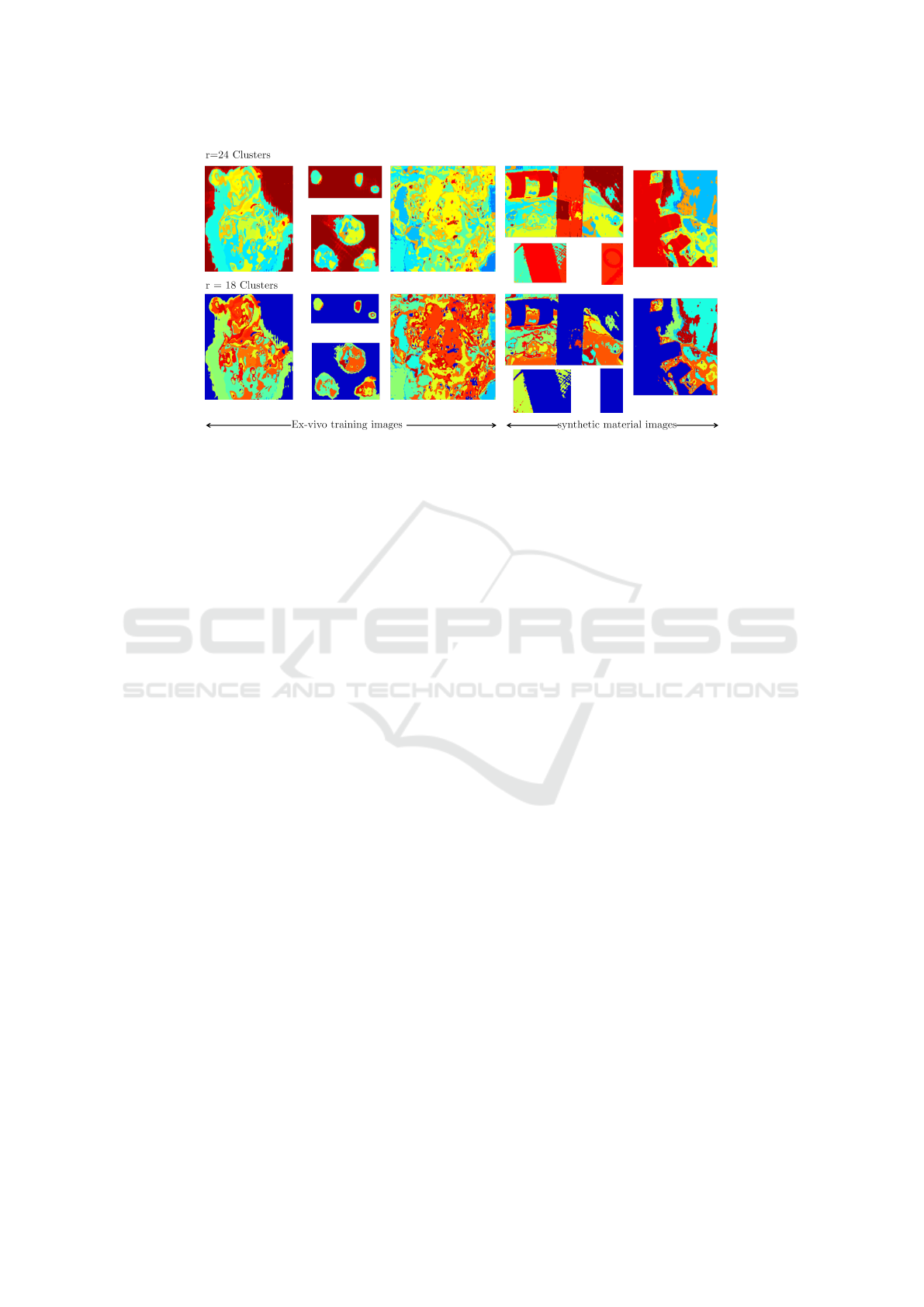
Figure 3: H2NMF clustering on the training set X
train
which consists of input ex-vivo tumor tissue HSI cube and on materials.
We in this case the ring on a cotton, and a cable in scene with open cranium and healthy tissues. This labeling with the
corresponding HSI cubes serves as the training set for constructing the random forest classifier.
ferent pure-pixels corresponding to different materi-
als The training set does not contain any in-vivo im-
ages since images containing the target tumor samples
shall remain unlabelled and not part of a class.
Test Set: The test set consists of both types of
images: Images ex-vivo of the tumor, and images in-
vivo from operations not in the training set. We refer
to the different test cubes/images as X
i
and their cor-
responding classification map by the random forest as
Y
i
.
We use algorithm (1) described in section 2 to per-
form hierarchical clustering of the training-images.
The principal goal here is to visualize the tissue struc-
ture as decomposed by the hierarchical clustering and
aid a surgeon or expert in annotating these images.
Another important goal is to determine the depth of
the hierarchy at which we are able to separate the
tumor, blood, tissues and materials and extract their
endmembers or spectral signatures.
3.1 Cluster Evaluation
In this section we compare the performance of
H2NMF, the clustering method used in our study,
with respect to other clustering algorithms: hier-
archical K-means(HKM), hierarchical spherical K-
means(HSKM). For the cases of NMF when used as
a clustering method, one does not explicitly use a dis-
tance function or dissimilarity (Kuang, 2014). The
prediction strength (Tibshirani and Walther, 2005) is
a well suited measure for cluster validation for NMF-
based clustering because it does not rely on a distance
function. Here we introduce a method similar to the
one described in (Kuang, 2014) to evaluate the NMF.
Given matrix X we split them into X
train
, X
train
over
which we obtain NMF decompositions, giving us
argminkX
train
−W
train
H
train
k
2
F
argminkX
test
−W
test
H
test
k
2
F
(4)
Now the prediction error can be obtained by solving
the non-negative least-squares problem for
H
predict
= argminkX
test
−W
train
Hk
2
F
(5)
We then compare the maximum abundance values in
H
test
, H
predict
to check which endmember index con-
tributed the most, and use this a measure of prediction
strength. This is because the H2NMF algorithm pro-
vides decomposition with one dominant endmember.
This is a variant on the classical prediction strength
measure (Tibshirani and Walther, 2005). We demon-
strate the results for the three hierarchical clustering
algorithms. The prediction strength provides us a way
to calculate the optimal number of clusters. Figure 4
demonstrates the prediction strength calculated over
random samples of the training set X
train
. This mea-
sure could also provide a reasonable guide in deter-
mining which clusters to split, aside the approxima-
tion error. We plot the maximum value of MRSA
from equation (3) for different number of clusters in
in figure 4. This demonstrates how far the pure-pixel
in cluster in a given level of hierarchy from its rank-2
NMF approximation. The figure also shows the plot
of the average approximation error in eq. 2 over dif-
ferent leaf sub-matrices for the three hierarchical clus-
tering algorithms. Both of these measures provide us
a tool to asses if the spectrum and sub-matrix at a leaf
are well approximated by a pure-pixel. Finally, we
evaluate the hierarchical clusters intrinsically by us-
ing the gap statistic (Tibshirani and Walther, 2005)
Unsupervised Clustering of Hyperspectral Images of Brain Tissues by Hierarchical Non-negative Matrix Factorization
81
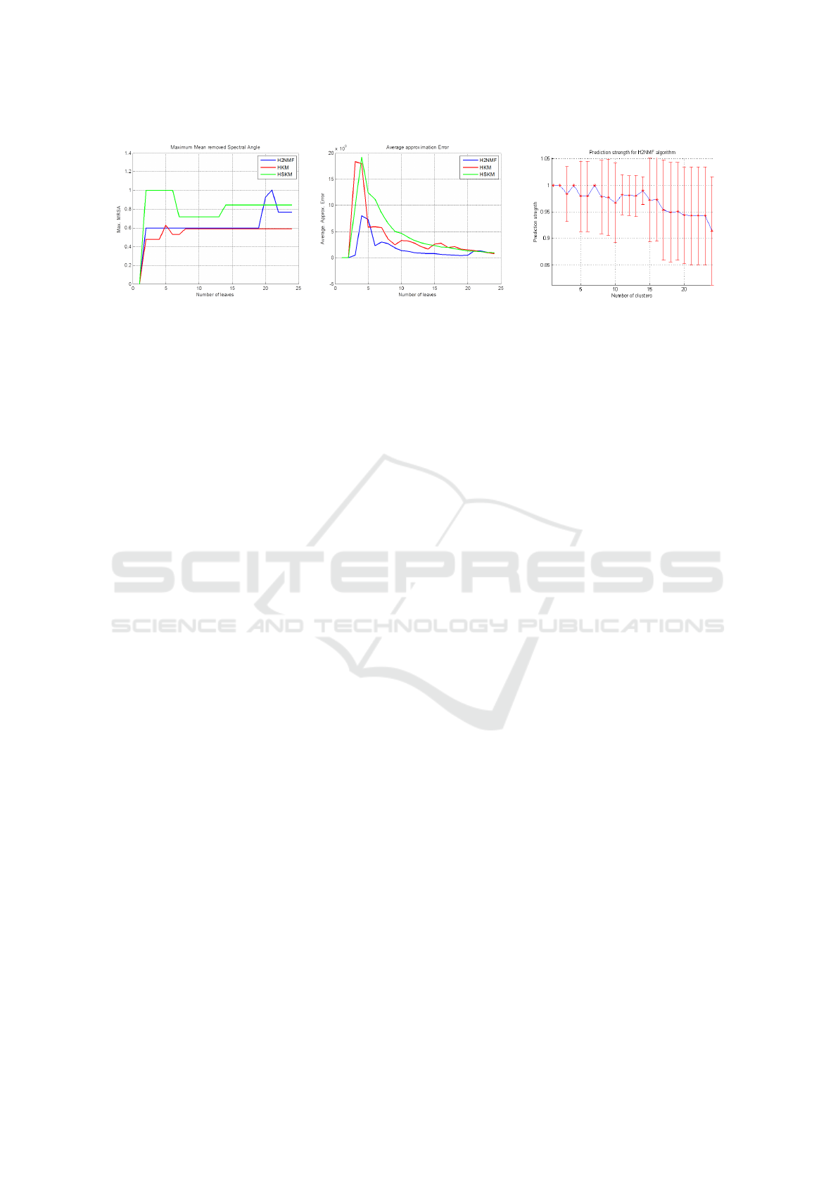
Figure 4: Left: the variation of the maximum MRSA(mean-removed spectral angle) to evaluate the homogeneity of clusters
in terms of endmember signature. This is evaluated across the three hierarchical clustering algorithms: H2NMF, HSKM,
HKM. We observe that all the three algorithms provide a good. Center: figure also shows the variation approximation error in
equation (2) with increasing leaves for three hierarchical clustering algorithms. Right: Plot demonstrating the mean prediction
strength calculated using the NMF decomposition. The red bars show the variance of the prediction strength. Optimal clusters
are chosen based on the maximum of the prediction strength. Here for example it is 14.
which using the average pairwise dissimilarity per
cluster to evaluate the number of clusters graphically,
by looking for an elbow.
We now train the resulting clustering on the train-
ing set X
train
. We use the Matlab’s implementation of
the random forest to train the Random forest(RF) with
the weak learner set to axis-aligned-hyperplane. We
first cut the subspace hierarchy by choosing the num-
ber of clusters r, and then use the clusters as labels to
train the RF-classifier.
The predictions of the RF-classifier are shown in
figure 5 when trained on two different levels of clus-
tering. We remark here that the actual subspace hi-
erarchy obtained by a sequence rank-2 NMF decom-
positions, is not completely approximated by the RF-
classifier. Nevertheless we do see a reasonable seg-
mentation. The rings shown in the in-vivo images
correspond to physical markers that were placed and
localize healthy and tumor tissues for evaluation pur-
poses. We do not obtain a single cluster label that
might correspond to tumor. To improve the classifi-
cation it would be ideal to integrate the structure of
the subspace hierarchy. This can be done by learning
a random forest for each level in the hierarchy. This
would of course be costly. A more principled solu-
tion would be to minimize an appropriate loss func-
tion that approximates the original subspace hierar-
chy.
The resulting segmentation from the classifier pro-
vides firstly the stable pure signatures of different ma-
terials in the ex-vivo tumors. The results are verified
basically by checking the presence of unique label (or
sets of labels) in a ring (1)) in the in-vivo images.
The tissue samples within these rings have been ver-
ified posteriori by pathology. One ring is assured to
surround a cancerous tissue sample, while the other
a healthy one. In this setup there was estimate of
the depth cancerous and its uniform exposure to the
VNIR-camera. This is tough to ensure during critical
surgeries. The color-map of the classification result in
figure 5 correspond to the color-map of the unsuper-
vised clustering in figure 3. The semantic meaning
of the labels is temporary and the color-map further
requires verification by a surgeon or pathology ex-
pert, to which finally a more sensible name shall be
attached. But it is evident that we are able to identify
plastic surgical materials, cotton.
4 ISSUES
Spectral Proximity of Benign and Malignant Tis-
sues: (Sahu et al., 2013) study differentiation be-
tween benign and malignant tumors in canine mam-
mary tumors, and detect tumors using a imaging spec-
trometer. Ovarian tissue characterization and tumor
differentiation (Utzinger et al., 2001), were performed
using NIR spectroscopy. The results showed that both
slope and intensity of reflectance spectra may have
the ability to discriminate normal from abnormal con-
ditions of the ovary. Slopes between 510 nm and
530 nm were most discriminatory for ovaries, while
630 nm to 900 nm in the study on kidneys (Peswani,
2007). The differences between malignant and benign
tissues in human breast tissues, have been attributed to
the metabolic difference due to the presence of more
oxy-hemoglobin, lipids and water. These elements
were used as the spectral markers considered for the
additive construction of the spectrum. (Kukreti et al.,
2010). This proximity in the spectral response of nor-
mal, benign and malignant tumor plays an crucial role
in classification of tumors pixels. In our study, due
the lack of information on the actual spectrum of tu-
mor tissues we are unable to provide a good division
BIOIMAGING 2016 - 3rd International Conference on Bioimaging
82
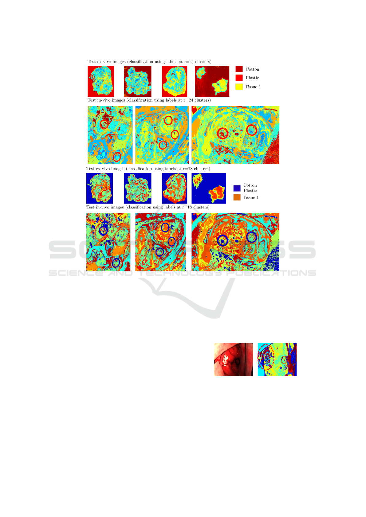
Figure 5: Results of the classification on the test set which consists of Ex-vivo images and In-vivo images test-set. Two sets
of classification maps are shown, the top image tile corresponding to learning the labels by cutting the subspace tree at r = 18
clusters and the bottom tile at r = 24. We observe that there are different tissue structures and materials found in the original
clustering in figure 3. It would be ideal to have a cluster/endmember corresponding to the tumor, though we remark that it
is not obvious to extract them or check for their existence. We can also notice that there are sets of labels co-occurring in
the marker rings though no trivial or consistent co-occurrence that can ensure a tumor detection. We can also notice in the
figure that certain materials have been approximated by the same subspace cluster: the cotton and the plastic. This can also be
visually confirmed by look at the subspace tree. Discriminating materials in this subspace tree structure is a crucial analysis
tool. As already mentioned, multiple classifiers are needed to approximate well the subspace clustering hierarchy. This would
merge the two levels of classification in this image into a more precise classification map.
of the subspace and the subsequent refinement of de-
cision boundary between normal and possible cancer-
ous tissue.
Specular Reflections. Specular reflections are a
prime problem in all our clustering and classification
steps and contributes to mis-classification. Specular
reflection occurs when the light source can be seen
as a direct reflection on the surface of the tissue un-
der study. The pixels affected by specular reflection
contain mainly the light source and may or may not
contain sufficient information on the reflectance of the
tissue under study. These reflected rays may also be
suspect of undergoing multiple reflections. An exam-
ple is shown in figure 6.
Figure 6: An in-vivo image and its classification map with
the specular reflection marked in dotted red ellipse. This
phenomena is not restricted to the optical range.
5 CONCLUSION
In this paper we applied and studied the hierarchi-
cal rank-2 NMF unmixing and clustering to segment
Unsupervised Clustering of Hyperspectral Images of Brain Tissues by Hierarchical Non-negative Matrix Factorization
83

brain tissue structure in an unsupervised setting. Sub-
sequently we have tried to train a random forest to
learn the structure of the subspace clusters.
Subspace Learning and Spatial Features:
Though the classifier can’t discriminate between nor-
mal tissues and tumor spectra, it provides a good seg-
mentation of the tissues and surgical materials in the
scene. The H2NMF hierarchy provides a hierarchy of
low rank sub-matrices that contain pure-pixels, and in
this case correspond to different brain tissues. This
cluster hierarchy can further be used by a surgeon in
loop to search more pertinent subspaces and feed the
results back to the classifier. We have seen the effect
of learning classifiers on different levels of the hier-
archical clustering. Though this produces reasonable
segmentations, it does not approximate the subspace
hierarchy exactly. We will study how to define loss
functions to encode this structure. Given that the dif-
ference in spectrum between tumor tissues and nor-
mal tissues are small, and prone to noise and varia-
tions across patients, building a robust spatial struc-
ture descriptor is important. One of the results of
our study points to the fact that the tissue structures
surrounding a tumor is a key feature. There is al-
ready evidence that in the micro-scale these normal
and cancerous tissues have a different toplogical ar-
rangement (Dvorak, 2003). This structural informa-
tion of tumor is useful to obtain a better detector for
cancerous tisues in hyperspectral images, since spec-
trum alone is not sufficient to classify them robustly.
Spatio-spectral features have been used in (Lu et al.,
2014), though our aim in the future is to use the spatial
features extracted by scattering-transform (Bruna and
Mallat, 2013) on the different abundance maps ex-
tracted by the hierarchical clustering algorithm. This
enables us to perform a principled search for features
across various scales.
ACKNOWLEDGEMENT
This work has been supported in part by the Euro-
pean Commission through the FP7 FET Open pro-
gramme ICT-2011.9.2, by the European Project HE-
LICoiD “HypErspectral Imaging Cancer Detection”
under Grant Agreement 618080.
REFERENCES
Bruna, J. and Mallat, S. (2013). Invariant scattering con-
volution networks. IEEE Trans. Pattern Anal. Mach.
Intell., 35(8):1872–1886.
Dvorak, H. F. (2003). How tumors make bad blood ves-
sels and stroma. The American journal of pathology,
162(6):1747–1757.
Gillis, N., Kuang, D., and Park, H. (2015). Hierarchi-
cal clustering of hyperspectral images using rank-two
nonnegative matrix factorization. IEEE T. Geoscience
and Remote Sensing, 53(4):2066–2078.
Gillis, N. and Luce, R. (2014). Robust near-separable
nonnegative matrix factorization using linear opti-
mization. Journal of Machine Learning Research,
15:1249–1280.
Kuang, D. (2014). Nonnegative matrix factorization for
clustering. PhD thesis, Georgia Institute of Technol-
ogy.
Kukreti, S., Cerussi, A. E., Tanamai, W., Hsiang, D.,
Tromberg, B. J., and Gratton, E. (2010). Characteriza-
tion of metabolic differences between benign and ma-
lignant tumors: High-spectral-resolution diffuse opti-
cal spectroscopy. Radiology, 254(1):277–284.
Liu, Z., Wang, H., and Li, Q. (2011). Tongue tumor de-
tection in medical hyperspectral images. Sensors,
12(1):162–174.
Lu, G. and Fei, B. (2014). Medical hyperspectral imaging:
a review. Journal of biomedical optics, 19(1):010901–
010901.
Lu, G., Halig, L., Wang, D., Qin, X., Chen, Z. G., and Fei,
B. (2014). Spectral-spatial classification for nonin-
vasive cancer detection using hyperspectral imaging.
Journal of biomedical optics, 19(10):106004–106004.
Ma, W.-K., Bioucas-Dias, J., Chan, T.-H., Gillis, N., Gader,
P., Plaza, A., Ambikapathi, A., and Chi, C.-Y. (2014).
A signal processing perspective on hyperspectral un-
mixing: Insights from remote sensing. Signal Pro-
cessing Magazine, IEEE, 31(1):67–81.
Panasyuk, S., Yang, S., Faller, D., Ngo, D., Lew, R., Free-
man, J., and Rogers, A. (2007). Medical hyperspectral
imaging to facilitate residual tumor identification dur-
ing surgery. Cancer Biol Ther, pages 439–46.
Peswani, D. L. (2007). Detection of Positive Can-
cer Margins Intra-operatively During Nephrectomy
and Prostatectomy Using Optical Reflectance Spec-
troscopy. ProQuest.
Sahu, A., McGoverin, C., Pleshko, N., Sorenmo, K., and
Won, C.-H. (2013). Hyperspectral imaging system
to discern malignant and benign canine mammary tu-
mors. In SPIE Defense, Security, and Sensing, pages
87190W–87190W. International Society for Optics
and Photonics.
Schulder, M. and Carmel, P. W. (2003). Intraoperative
magnetic resonance imaging: impact on brain tumor
surgery. Cancer Control, 10(2):115–124.
Tibshirani, R. and Walther, G. (2005). Cluster validation
by prediction strength. Journal of Computational and
Graphical Statistics, 14(3):511–528.
Utzinger, U., Brewer, M., Silva, E., Gershenson, D., Blast,
R. C., Follen, M., and Richards-Kortum, R. (2001).
Reflectance spectroscopy for in vivo characterization
of ovarian tissue. Lasers in surgery and medicine,
28(1):56–66.
BIOIMAGING 2016 - 3rd International Conference on Bioimaging
84
