Controlling the Cost of Prediction in using a Cascade of Reject Classifiers
for Personalized Medicine
Blaise Hanczar
1
and Avner Bar-Hen
2
1
IBISC, IBGBI University of Evry, 23 bd de France, 91034 Evry, France
2
MAP5, University Paris Descartes, 45 rue des saint-peres 75006 Paris, France
Keywords:
Supervised Learning, Reject Option, Cascade Classifier, Genomics Data, Personalized Medecine.
Abstract:
The supervised learning in bioinformatics is a major tool to diagnose a disease, to identify the best therapeutic
strategy or to establish a prognostic. The main objective in classifier construction is to maximize the accuracy
in order to obtain a reliable prediction system. However, a second objective is to minimize the cost of the use
of the classifier on new patients. Despite the control of the classification cost is high important in the medical
domain, it has been very little studied. We point out that some patients are easy to predict, only a small subset
of medical variables are needed to obtain a reliable prediction. The prediction of these patients can be cheaper
than the others patient. Based on this idea, we propose a cascade approach that decreases the classification cost
of the basic classifiers without dropping their accuracy. Our cascade system is a sequence of classifiers with
rejects option of increasing cost. At each stage, a classifier receives all patients rejected by the last classifier,
makes a prediction of the patient and rejects to the next classifier the patients with low confidence prediction.
The performances of our methods are evaluated on four real medical problems.
1 INTRODUCTION
The personalized medicine is an ongoing revolution
in medicine; its objective is to maximize the wellness
for each individual rather than simply to treat disease.
According to Hood and Friend (Hood and Friend,
2011), this revolution is based on several points. The
first one is to consider that medicine is an informa-
tion science. The second point is the emergence of
technologies that will let us explore new dimensions
of patient data space, like the ”omics” technologies.
The last point is the development of powerful new
mathematical and computational methods, specially
in machine learning, that will let us analysis the marge
amount of data associated with each individual. To-
day physicians have access to a large amount data for
each patient from different sources: clinical, environ-
mental, psychological, biologic or omic. The use of
automated methods is indispensable to analyse and
extract relevant information from these data. An im-
portant way of research is the development of predic-
tion systems whose objectives generally are to diag-
nose a disease, to identify the best therapeutic strat-
egy or to establish a prognostic for a patient. These
systems, called classifiers, are constructed from su-
pervised learning methods, the most popular are the
discriminant analysis (Dudoit et al., 2002), the sup-
port vector machine (Furey et al., 2000), the random
forest (Diaz-Uriarte and Alvarez de Andres, 2006),
the neural networks (Khan et al., 2001) or the en-
semble methods (Yang Pengyi; Hwa Yang Yee; Bing
B. Zhou;, 2010).
The primordial objectiveof the prediction systems
is to maximize their accuracy in order to obtain reli-
able predictions. However, a second objective, gen-
erally ignored in research studies, is to minimize the
cost of the prediction. In a classifier, a patient is rep-
resented by a set of variables. These variables come
from different medical exams and each of these ex-
ams has a cost. The use of a classifier requires the
values of all variables of the patient; the cost of the
prediction is the sum of the costs of all exams used
by the classifier. Note that the cost does not neces-
sary represent money, it may also represent time, sec-
ondary effects of treatment or any other non-infinite
resource. In practice, a good prediction system has to
both maximize its accuracy and minimize its cost.
In this paper we propose a new method that re-
duce the prediction cost without increasing the error
rate. In prediction problems, it is worth to note that
some patients are easier to predict than others and
do not need all medical exams. For these patients,
a reliable prediction can be done with a small sub-
42
Hanczar, B. and Bar-Hen, A.
Controlling the Cost of Prediction in using a Cascade of Reject Classifiers for Personalized Medicine.
DOI: 10.5220/0005685500420050
In Proceedings of the 9th International Joint Conference on Biomedical Engineering Systems and Technologies (BIOSTEC 2016) - Volume 3: BIOINFORMATICS, pages 42-50
ISBN: 978-989-758-170-0
Copyright
c
 2016 by SCITEPRESS – Science and Technology Publications, Lda. All rights reserved

set of variables and can be therefore less expensive.
Based on this observation, we propose a new super-
vised classification approach using a cascade of clas-
sifiers with reject option. This cascade is a sequential
set of classifiers with reject option of increasing cost.
The patient data are submitted to the first classifier
that makes a prediction. If this prediction is judged
not reliable, the patient is rejected to the next classi-
fier of the cascade needing additional variables. The
process is repeated until a reliable prediction has been
done. This approach allows reducing the cost of the
basic classifier using all variables. In this approach,
there is a trade-off between the accuracy and the cost
of the predictions. The two main scientific keys of
our method are the computation of the rejection area
of all classifiers of the cascade. The second is to find
the optimal order of the variables that form the struc-
ture of the cascade. The section two gives the state
of the art of cost minimization methods and cascade
classification. In section three, we provide the formu-
lation of the classification with rejection option and
the cascade. The two algorithms for the computation
of the rejection areas and the order of the variables are
given in detail. The section four presents the results
on four real datasets and analysis the performance of
our method.
2 RELATED WORK
The reduction prediction cost problem is close to the
active feature acquisition problem in the cost sensitive
learning (Saar-Tsechansky et al., 2009). The objec-
tive is sequentially decided if we want to acquire the
next feature in order to increase the accuracy of the
classifier. Markov decision process is one of the usual
approach used in this context, for example, Kapoor
(Kapoor and Horvitz, 2009) propose a new class of
policies inspired from active learning. Tan propose
an attribute value acquisition algorithm driven by the
expected cost saving of acquisition only for support
vector machine (Tan and yen Kan, 2010). Nan devel-
oped a variant of random forest dealing with the cost
of the variables (Nan et al., 2015).
One simple structure for incorporating the cost
into learning is through a cascade of classifiers. This
approach has been popularized by Viola and Jones
(Viola and Jones, 2004) with their detection cascade
used in image analysis for object detection. Cheap
variables are used to discard examples belonging to
the negative class. This type of method is focused on
unbalanced data with very few positive examples and
a large number of negative examples. Note that the
main objective of this Viola’s cascade is to increase
the accuracy of the prediction, they do not deal with
the prediction cost. In the context of information re-
trieval, Wang adapted the cascades to ranking and in-
corporated variables costs but retained the underlying
greedy paradigm (Wang et al., 2011). Raykar et al.
(Raykar et al., 2010) explore the idea of a cascade of
reject classifier. Their version is a soft cascade where
each stage accepts or rejects examples according to a
probability distribution induced by the previous stage.
Each stage of the cascade is limited to linear clas-
sifiers, but they are learned jointly and take in ac-
count of the cost of the variables. Trapeznikov and
Saligrama (Trapeznikov and Saligrama, 2013) pro-
pose a multi-stage multi-class system where the reject
decision at each stage is posed as a supervised binary
classification problem. They derive bound for VC di-
mension to quantify the generalization error.
A common limitation of all these methods is that
the order of the variables is supposed to be known.
The structure of the cascade is therefore fixed. Our
method overcomes these limitations in using a heuris-
tic to compute an order of the variables.
3 CASCADE OF REJECT
CLASSIFIERS FORMULATION
3.1 Formulation of the Problem
We consider a classification problem with two classes
(positive ”1” and negative ”0”) with D variables
{v
1
, ...,v
D
}. Let’s a training set of N examples T =
{(x
1
, y
1
), ..., (x
N
, y
N
)} where x
i
∈ R
D
is the variable
vector and y
i
∈ {0, 1} is the label. We denote c
i
the
cost for acquiring the i-th variable of an example.
Let’s Ψ : R
D
→ {0, 1} the basic classifier constructed
from a usual supervised learning procedure and mak-
ing predictions in using all variables. Our objective is
to construct a cascade that obains better performances
than the basic classifier.
In this context, the performance of a classifier is
measured by two values: its error rate i.e. the prob-
ability that the prediction does not correspond to the
true label, noted E = p(Ψ(x) 6= y) and its cost that
is the total acquisition cost of all variables required
by the classifier, noted C =
∑
d
i=1
c
i
. These values are
combined into a new value called loss, that represent
the total performance of the classifier and is defined
by:
L = C + ΛE (1)
Λ is a parameter that represented the penalty of a mis-
classification. In our cascade, this parameter controls
the trade-off between the cost and the error rate. For
Controlling the Cost of Prediction in using a Cascade of Reject Classifiers for Personalized Medicine
43

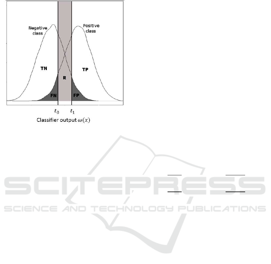
Figure 1: Distribution of the classes on the classifier out-
put. TP, TN, FP, FN and R represent respectively the true
positive, true negative, false positive, false negative and re-
jection area.
the basic classifier, the cost C is constant since we al-
ways have to pay all variables. The objective is to
construct a cascade with a loss lower than the loss of
the basic classifier.
3.2 Classifier with Rejection Option
The base element of our cascade system is the clas-
sifier with reject option. This type of classifier can
reject examples if it is not enough confident in the
predictions. No class is assigned to rejected exam-
ples. Let’s Ψ a classifier whose the output ω(x) is a
continuous value. In fixing a threshold t on this out-
put, we define a classic classifier that assigns one of
the two classes to each example. In fixing two thresh-
olds {t
0
,t
1
}, we define a classifier that rejects some
examples and assigns one of the two classes to the
non-rejected examples.
Ψ(x) =



0 if ω(x) ≤ t
0
1 if ω(x) ≥ t
1
R if t
0
< ω(x) < t
1
(2)
with the constraint t
0
≤ t
1
. R represents the rejec-
tion of the example x. Figure 1 shows the distribution
of the two classes on the classifier output. The two
thresholds t
0
and t
1
divide the classifier output into
three decision regions ({Ψ(x) = 1, Ψ(x) = 0, Ψ(x) =
R}). The performance of the classifier depends on
the following values: the error rate E = p(Ψ(x) 6=
y, Ψ(x) 6= R) (represented by the FP and FN areas in
the figure 1), the penalty of an error λ
E
, the accuracy
A = p(Ψ(x) = y) (represented by the TP and TN ar-
eas), the penalty of a good classification λ
A
, the rejec-
tion rate R = p(Ψ(x) = R) (represented by the R area)
and the penalty of a rejection λ
R
. Note that we have
A+ R+ E = 1. The performance of a reject classifier
is measured by its expected loss:
L(Ψ) = λ
A
A+ λ
E
E + λ
R
R (3)
The objective is to find the thresholds t
0
and t
1
minimizing the expected loss of the classifier. For that
we use the Chow’s rule (Chow, 1970) that consider
a Bayesian scenario where the output of the classi-
fiers is the posterior probability of the positive class
ω(x) = p(1|x). Let’s the three loss functions L
1
, L
0
and L
R
that represent the expected loss that is obtained
in assigning an example x to respectively the class 1,
0 or R.
L
1
(x) = λ
A
ω(x) + λ
E
(1− ω(x)))
L
0
(x) = λ
E
ω(x) + λ
A
(1− ω(x))
L
R
(x) = λ
R
(4)
From these formulas we can compute directly the
optimal decision thresholds in solving the equations
L
1
(x)
L
R
(x)
= 1 ⇒ t
∗
1
=
λ
R
− λ
E
λ
A
− λ
E
L
0
(x)
L
R
(x)
= 1 ⇒ t
∗
0
=
λ
R
− λ
A
λ
E
− λ
A
(5)
3.3 Cascade of Reject Classifiers
Our cascade system is a sequence of D classifiers with
reject option Ψ
1
, ..., Ψ
D
of increasing cost, illustrated
by the figure 2. The i-th classifier Ψ
i
receives all ex-
amples rejected by the classifier Ψ
i−1
, makes predic-
tions and sends all rejected examples to Ψ
i+1
. The last
classifier Ψ
D
has no reject option and makes a predic-
tion for all received examples. The first classifier Ψ
1
receives all examples. For the moment, we consider
that the order of the variables is fixed, the classifier Ψ
i
uses only the i first features so its cost is
∑
i
j=1
c
j
. For
each classifier Ψ
i
, its error rate E
i
, accuracy A
i
and
rejection rate R
i
are computed as :
E
i
= p(Ψ
i
(x) 6= y, Ψ
i
(x) 6= R|Ψ
j
(x) = R ∀ j ∈ [1, i− 1])
A
i
= p(Ψ
i
(x) = y|Ψ
j
(x) = R ∀ j ∈ [1, i− 1])
R
i
= p(Ψ
i
(x) = R|Ψ
j
(x) = R ∀ j ∈ [1, i− 1])
(6)
From these formulas, we can define the loss L
i
of
each classifier of the cascade by a weighted combi-
nation of their error rate, accuracy and rejection rate.
The weight of a good classification is the cost of the
used variables, the weight of an error is the cost of
BIOINFORMATICS 2016 - 7th International Conference on Bioinformatics Models, Methods and Algorithms
44

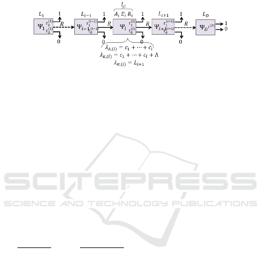
Figure 2: Cascade of D reject classifiers.
the used variables plus the penalty of misclassifica-
tion. When an example is rejected, it is sent to the
next classifier so the weight of rejection is the loss of
the next classifier L
i+1
. The loss of an entire cascade
L can be computed recursively by:
L = L
1
L
i
= A
i
i
∑
j=1
c
j
+ E
i
(
i
∑
j=1
c
j
+ Λ) + R
i
L
i+1
L
D
= A
D
D
∑
j=1
c
j
+ E
D
(
D
∑
j=1
c
j
+ Λ)
(7)
The optimization of the cascade consist of find-
ing the optimal rejection areas of each classifier that
minimize the loss of the cascade. For each classi-
fier of the cascade, the rejection area i.e. the thresh-
olds t
0
and t
1
, can be computed in using the Chow’s
rule. For the classifier Ψ
i
the penalty of a good clas-
sification is λ
A
=
∑
i
j=1
c
j
, the penalty of an error is
λ
E
=
∑
i
j=1
c
j
+ Λ and the penalty of a rejection is
λ
R
= L
i+1
. In using the formulas (5) we obtain the
optimal rejection area of the classifier Ψ
i
.
t
∗
0,(i)
=
L
i+1
−
∑
i
j=1
c
j
Λ
t
∗
1,(i)
=
∑
i
j=1
c
j
+ Λ − L
i+1
Λ
(8)
Unfortunately, we can not simply use these formu-
las on each classifier to obtain the optimal cascade.
The problem is that the classifiers and their perfor-
mances are depending each other. When a new re-
jection area of a classifier is computed, the sets of
examples rejected to the next classifiers change, the
performances of the next classifiers and their penal-
ties of rejection change too. A new rejection area
has, therefore, to be computed. All rejection areas,
performances and penalties of all classifiers are circu-
larly dependent. To solve this optimization problem
we propose a heuristic described in the algorithm 1.
The cascade is initialized as the basic classifier i.e.
all classifiers reject all examples and all examples are
sent to the last classifier using all variables. The iter-
ative procedure contains three steps. The first one is
to compute the accuracy, error rate and rejection rate
of all classifiers. Then the penalties of rejection of
all classifiers (excepted the last one) are computed in
using the formula (7). The penalty of rejection de-
pends on the performances of the next classifier, the
penalties are therefore computed from the classifier
Ψ
D−1
to the classifier Ψ
1
. Finally, the two rejection
thresholds are computed for each classifier from the
penalties of good classification, misclassification, and
rejection. This procedure is iterated MaxIter times,
MaxIter is a parameter to be chosen by the users. In
the results section, we investigate empirically the im-
pact of this parameter and select MaxIter = 10.
3.4 Order of the Variables
In the previous section, we considered that the order
of the variables in the cascade was fixed, but in real
case the variable order is rarely known. The perfor-
mance of the cascade depend highly on the order, we
want the most informative and less expensive vari-
ables at the beginning and the less informative and
most expensive at the end. The usefulness of a vari-
able is not correlated to its cost and is depending on
the variable selected in the previous classifiers. For
these reasons, it is not easy to compute the quality of
the variables and determine their position in the cas-
cade. One solution is to test all orders and select the
one that produce the best cascade. However, there
are D! possible orders, this method is intractable for
D > 10. We propose a heuristic, in the algorithm 2,
that selects an order of the variable. The heuristic be-
gins with an empty set of variables and selects one by
one each variable. At each iteration i, i− 1 variables
have been already selected and are used to construct
a cascade of size i− 1. All non-selected variables are
tested to form the i-th stage of the cascade. We select
the variable that minimizes the loss of the cascade.
The procedure is iterated until all variables have been
selected.
Controlling the Cost of Prediction in using a Cascade of Reject Classifiers for Personalized Medicine
45

Algorithm 1: Optimization algorithm of the reject areas.
1: procedure REJECT AREAS OPTIMIZATION
2: // Initialization
3: for i from 1 to D− 1 do
4: t
0,(i)
← 0; t
1,(i)
← 1
5: end for
6: t
0,(D)
← 0.5; t
1,(D)
← 0.5
7: for nbiter from 1 to MaxIter do
8: // Computation of the reject classifiers
performances
9: L ← newL
10: for i from 1 to D do
11: A
(i)
← accuracy ofΨ
i
12: E
(i)
← error rate ofΨ
i
13: R
(i)
← rejection rate ofΨ
i
14: end for
15: // Computation of the rejection costs
16: λ
D
← 0
17: for i from D− 1 to 1 do
18: λ
R,(i)
← A
(i+1)
∑
i+1
j=1
c
j
+
E
(i+1)
(
∑
i+1
j=1
c
j
+ Λ) + R
(i+1)
λ
R,(i+1)
19: end for
20: // Computation of the thresholds
21: for i from 1 to D− 1 do
22: (t
0,(i)
,t
1,(i)
) computed from the cost
λ
G
=
∑
i
j=1
c
j
, λ
E
=
∑
i
j=1
c
j
+ Λ and λ
R
= λ
R,(i)
23: end for
24: end for
25: return (t
0,(i)
,t
1,(i)
) ∀i ∈ [1, D− 1]
26: end procedure
Algorithm 2: Selection of the variables order.
1: procedure REJECT AREAS OPTIMIZATION
2: V ← {v
1
, ..., v
D
}
3: Order ←
/
0
4: for j from 1 to D do
5: best.L ← Λ
6: for i from 1 to D− j + 1 do
7: Tested.Order ← concat(Order,V[i])
8: Construction of the cascade from
Tested.Order
9: L ← loss of the cascade
10: if L < best.L then
11: best.L ← L, best.V ← V[i]
12: end if
13: end for
14: Order ← Order + best.V
15: V ← V − best.V
16: end for
17: return Order
18: end procedure
4 EXPERIMENTS AND RESULTS
4.1 Study Design and Datasets
We perform a set of experiments to investigate the
performance of our cascade method. For these ex-
periments, we use several real medical and genomic
datasets. The first one is the pima dataset (Smith et al.,
1988) whose the objective is to predict signs of dia-
betes of 768 patients based on eight clinical variables.
We select this dataset because the costs of variables
are provided, this information is very rare in the pub-
lic datasets. The second one is the Wisconsin Diag-
nostic Breast Cancer (wdbc) datasets whose the ob-
jective is to differentiate the malignant tumors from
benign tumors of 569 patients based on 30 medical
variables. Since the costs of variables were no avail-
able, we randomly draw from a uniform distribution
U[0, 1] the cost of the variables. The third one is the
lung cancer dataset (Bhattacharjee, 2001) whose the
objective is to identify the adenocarcinoma from the
other type of tumor based on the several thousand of
gene expression. The last one is the prostate cancer
dataset (Singh et al., 2002) whose the objective is to
diagnosis cancer from safe tissues based on the sev-
eral thousand of gene expression of 339 patients. For
the two last datasets, since all gene expressions have
been measured simultaneously with microarrays, the
costs of all variables are equal. For all datasets, we
normalize the costs of the variables such that the sum
of all costs is 1. The basic classifier using all variables
pays, therefore, one for each example.
We tested our method with two classification al-
gorithms: the linear discriminant analysis (LDA) and
the support vector machine (SVM) with a radial ker-
nel. For high dimensional datasets, like the lung and
prostate cancer dataset, a feature selection step is in-
cluded in the classification in order to reduce the num-
ber of variables. We have used a filter method based
on the t-test score to select the best variables. Note
that the variable selection is performed in the classi-
fier construction in order to avoid any selection bias
(Ambroise and McLachlan, 2002).
The objective of our method is to reduce the clas-
sification cost and have a lower loss than the basic
classifier. We, therefore, compare the performances
of our cascade of the performance of the basic classi-
fiers. One of the key points of the cascade construc-
tion is the selection of the variables order for which
we have proposed a heuristic (algo 2). In order to
show the usefulness of our heuristic, we compare our
method to the performance of cost based order cas-
cade. In the cost-based order cascade, the variables
are ordered by their increasing cost. The cascade be-
BIOINFORMATICS 2016 - 7th International Conference on Bioinformatics Models, Methods and Algorithms
46

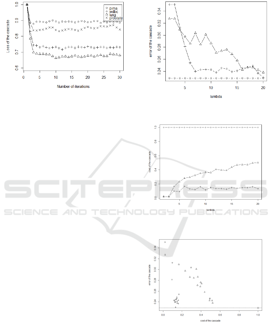
Figure 3: Loss of the cascade during the computation of the
rejection areas.
gins with the cheapest variables and finishes with the
more expensive.
4.2 Sensitivity Analysis
Our method depends on two parameters: the number
of iterations in the heuristic of rejection areas compu-
tation MAXITER and the penalty of an error Λ. We
investigate the impact of these two parameters on the
behavior of our method.
The figure 3 shows the loss of the cascade during
the heuristic of the rejection areas computation for the
four datasets with the LDA classifier. The loss values
have been normalized such that all curves are plotted
in the same graphics, we set the loss of the cascade at
its initialization to 1. The figure shows that the cas-
cade convergesquickly toward a stable solution for all
datasets. Moreover, we see that the loss of the solu-
tion is much lower than the loss of initialization. This
last point shows that our heuristic provides good re-
jection areas for the cascade. According to these re-
sults, we choose to set MAXITER = 10, this value is
enough to reach a stable solution and limits the com-
putation time of cascade learning.
The figures 4, 5 and 6 gives respectively the error
rate vs λ, the cost of the cascade vs Λ and the cost
vs the error rate with the pima dataset and the LDA
classifier. We do not have the space to put the graph-
ics of the other datasets and classifiers, but they are
similar to these figures and lead to the same conclu-
sions. The dot represents the basic classifier, the trian-
gle line is the cost based order cascade and the cross
line is the heuristic based order cascade. Λ is increas-
ing with the cost of the cascade and decreasing with
its error rate. Λ controls the trade-off between the er-
ror rate and the variable cost. For a low value of Λ, the
misclassifications are more tolerated, fewer variables
are therefore needed, but the error rate increases. At
the extreme, Λ ≤ 2 in these figures, the cascade keeps
:basic classifier, △:cost based, +:heuristic based
Figure 4: Error rate of the cascade in function on Λ.
:basic classifier, △:cost based, +:heuristic based
Figure 5: Cost of the cascade in function on Λ.
:basic classifier, △:cost based, +:heuristic based
Figure 6: Error of the cascade in function on prediction cost.
The performances are presented by a set of points because
their are depending on the value of the parameter Λ.
only the first variable for all examples. For a high
value of Λ, the misclassifications are very penalized,
the cascade needs more variables in order to get more
Controlling the Cost of Prediction in using a Cascade of Reject Classifiers for Personalized Medicine
47

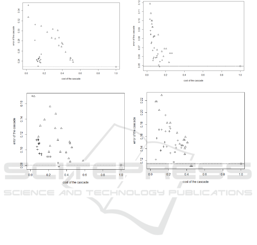
pima wdbc
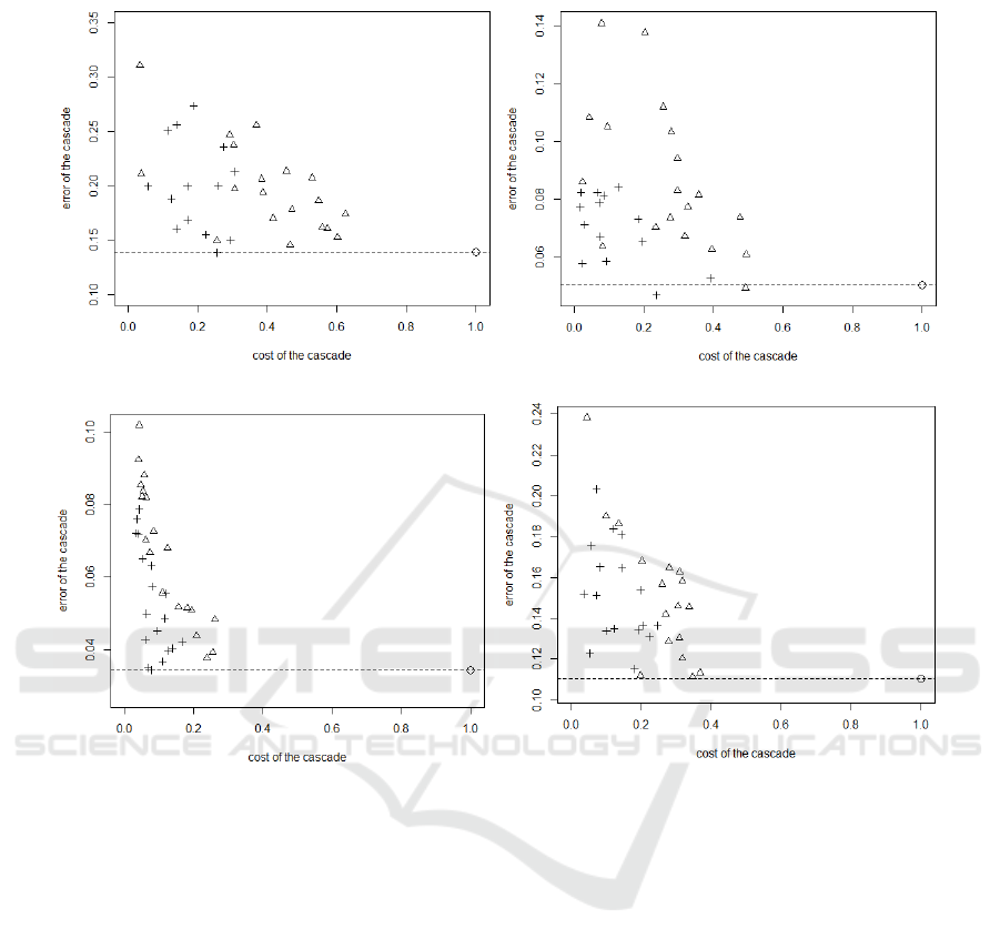
lung cancer prostate cancer
Figure 7: Classification cost vs Error rate plots for all datasets with linear discriminant analysis. The performances are
presented by a set of points because their are depending on the value of the parameter Λ.
information and minimize the risk of error. We see
that the error rate of the cascade is never lower than
the error rate of the basic classifier. That is logic since
the basic classifier uses all information, i.e. all vari-
ables for all examples. The error rate of the cascade
can be only higher or equal than the error of the ba-
sic classifier. Note that there is always a value of Λ
where the error rate of the cascade reaches the error
rate of the basic classifier. In the figure 4, it is Λ = 20
for heuristic based order cascade and Λ > 20 for cost
based order cascade. This point is interesting because
it corresponds to a cascade that does not decrease the
accuracy of the classifier. Let focus on the behavior
of the cost based order cascade (triangle curve) in the
loss figure. For low values of Λ, the loss of cost based
order cascade is the same than heuristic based order
cascade, for high values of Λ it reaches the loss of ba-
sic classifier. The reason is that the cost based order
cascade favors cheap variables, for low values of Λ
the cost of the cascade is more important than its er-
ror rate, the cost based order cascade is therefore well
adapted.
4.3 Classification Results
The figures 7 and 8 show the classification cost vs
error rate plot for all datasets with the linear discrim-
inant analysis. In these graphics, the closest a point
is from the left bottom corner, the better the perfor-
mance is. The dot represents the performance of the
basic classifier, its cost is 1 by definition and its er-
ror rate is represented by the dotted line. The trian-
gles and the crosses represent respectively the perfor-
mance of the cost based order cascade and the heuris-
tic based order cascade. The performances are pre-
sented by a set of points because their are depending
on the value of the parameter Λ. In all graphics, we
see that the cascade can decreases strongly the cost of
the classification. With the same accuracy as the ba-
sic classifier, we can reduce the cost by 85% for pima
datasets, 86% for wdbc dataset, 70% for the lung can-
cer dataset and 74% for prostate cancer datatset with
the LDA classifier and by 74% for pima datasets, 73%
for wdbc dataset, 90% for the lung cancer dataset and
80% for prostate cancer datatset with the SVM classi-
BIOINFORMATICS 2016 - 7th International Conference on Bioinformatics Models, Methods and Algorithms
48

pima wdbc
lung cancer prostate cancer
Figure 8: Classification cost vs Error rate plots for all datasets with support vector machine. The performances are presented
by a set of points because their are depending on the value of the parameter Λ.
fier. This cost can again be decreased, if we accept to
increase the error rate. We also see that in all graphics
that the triangles clearly dominate the crosses. This
means that the heuristic based order cascade outper-
forms the cost based order cascade.
5 CONCLUSIONS
The cascade methods are very promising for person-
alized medicine since the prediction system and its
cost are adapted to each patient. There are some prob-
lems. The first one is the problem of high dimension
data like the omics data. If the number of variables is
very high (several thousand and more) the heuristic of
order selection is computationally intractable. In the
current work, we deal with this problem in making a
classic variable selection step before the construction
of the cascade. A more efficient solution would be to
perform the selection in taking account of the variable
cost and during the construction of the cascade. The
second question is the problem of cost based prob-
lems. In the current work the costs are unique and
fixed for each variable. In another context they may
have several costs, for example, the medical exam to
obtain some variables may have a cost in money, du-
ration and a risk of secondary effect. All these costs
impact the performance of the cascade. They may
also have interactions between the costs. The cost of
a variable v
i
can decrease if a variable v
j
has already
been measured. We will study these new interesting
problems on future works.
REFERENCES
Ambroise, C. and McLachlan, G. (2002). Selection bias in
gene extraction on the basis of microarray gene ex-
pression data. Proc. Natl. Acad. Sci., 99(10):6562–
6566.
Bhattacharjee, A. (2001). Classification of human
Controlling the Cost of Prediction in using a Cascade of Reject Classifiers for Personalized Medicine
49

lung carcinomas by mRNA expression profiling re-
veals distinct adenocarcinoma subclasses. PNAS,
98(24):13790–5.
Chow, C. (1970). On optimum recognition error and reject
tradeoff. IEEE Transactions on Information Theory,
16(1):41–46.
Diaz-Uriarte, R. and Alvarez de Andres, S. (2006). Gene
selection and classification of microarray data using
random forest. BMC Bioinformatics, 7(3).
Dudoit, S., Fridlyand, J., and Speed, P. (2002). Compari-
son of discrimination methods for classification of tu-
mors using gene expression data. Journal of American
Statististial Association, 97:77–87.
Furey, T., Cristianini, N., Duffy, N., Bednarski, D., Schum-
mer, M., and Haussler, D. (2000). Support vector
machine classification and validation of cancer tissue
samples using microarray expression data. Bioinfor-
matics, 16(10):906–914.
Hood, L. and Friend, S. H. (2011). Predictive, personalized,
preventive, participatory (p4) cancer medicine. Nat
Rev Clin Oncol, 8(3):184–187.
Kapoor, A. and Horvitz, E. (2009). Breaking boundaries:
Active information acquisition across learning and di-
agnosis. Advances in neural information processing
systems.
Khan, J., Wei, J., Ringner, M., Saal, L., Ladanyi, M., West-
ermann, F., Berthold, F., Schwarb, M., Antonescu, C.,
Peterson, C., and Meltzer, P. (2001). Classification
and diagnostic prediction of cancers using gene ex-
pression profiling and artificial neural networks. Na-
ture Medecine, 7:673–679.
Nan, F., Wang, J., and Saligrama, V. (2015). Feature-
budgeted random forest. International Conference on
Machine Learning.
Raykar, V. C., Krishnapuram, B., and Yu, S. (2010). De-
signing efficient cascaded classifiers: tradeoff be-
tween accuracy and cost. In Proceedings of the 16th
ACM SIGKDD international conference on Knowl-
edge discovery and data mining, pages 853–860.
ACM.
Saar-Tsechansky, M., Melville, P., and Provost, F. (2009).
Active feature-value acquisition. Management Sci-
ence, 55(4):664–684.
Singh, D., Febbo, P., Ross, K., Jackson, D., Manola, J., and
Ladd, C. (2002). Gene expression correlates of clini-
cal prostate cancer behavior. Cancer Cell., 1(2):203–
209.
Smith, J. W., Everhart, J., Dickson, W., Knowler, W., and
Johannes, R. (1988). Using the adap learning algo-
rithm to forecast the onset of diabetes mellitus. In Pro-
ceedings of the Annual Symposium on Computer Ap-
plication in Medical Care, page 261. American Med-
ical Informatics Association.
Tan, Y. F. and yen Kan, M. (2010). Cost-sensitive attribute
value acquisition for support vector machines. Tech-
nical report, National University of Singapore.
Trapeznikov, K. and Saligrama, V. (2013). Supervised se-
quential classification under budget constraints. In
Proceedings of the Sixteenth International Conference
on Artificial Intelligence and Statistics, pages 581–
589.
Viola, P. and Jones, M. J. (2004). Robust real-time face
detection. International journal of computer vision,
57(2):137–154.
Wang, L., Lin, J., and Metzler, D. (2011). A cascade
ranking model for efficient ranked retrieval. In Pro-
ceedings of the 34th International ACM SIGIR Con-
ference on Research and Development in Information
Retrieval, SIGIR ’11, pages 105–114, New York, NY,
USA. ACM.
Yang Pengyi; Hwa Yang Yee; Bing B. Zhou;, B. B. Z.
(2010). A review of ensemble methods in bioinfor-
matics. Current Bioinformatics, 5(4):296.
BIOINFORMATICS 2016 - 7th International Conference on Bioinformatics Models, Methods and Algorithms
50