
Camera Placement Optimization Conditioned on Human Behavior and
3D Geometry
Pranav Mantini and Shishir K. Shah
Department of Computer Science, University of Houston, 4800 Calhoun Road, Houston, Texas, U.S.A.
Keywords:
Camera Placement Optimization, Human Motion Forecasting, Occupancy Map Estimation, Face Detection,
Human Activity, Effective Surveillance.
Abstract:
This paper proposes an algorithm to optimize the placement of surveillance cameras in a 3D infrastructure.
The key differentiating feature in the algorithm design is the incorporation of human behavior within the in-
frastructure for optimization. Infrastructures depending on their geometries may exhibit regions with dominant
human activity. In the absence of observations, this paper presents a method to predict this human behavior
and identify such regions to deploy an effective surveillance scenario. Domain knowledge regarding the in-
frastructure was used to predict the possible human motion trajectories in the infrastructure. These trajectories
were used to identify areas with dominant human activity. Furthermore, a metric that quantifies the position
and orientation of a camera based on the observable space, activity in the space, pose of objects of interest
within the activity, and their image resolution in camera view was defined for optimization. This method was
compared with the state-of-the-art algorithms and the results are shown with respect to amount of observable
space, human activity, and face detection rate per camera in a configuration of cameras.
1 INTRODUCTION
Video surveillance is an integral part of many pub-
lic areas such as airports, banks and train stations.
The positioning and orientation of the cameras can
play a significant role in enabling effective surveil-
lance needs such as face detection, tracking, etc. The
geographic distribution of cameras to enable effective
surveillance can be scenario specific. For example, in
a movie theater, it might be sufficient to deploy cam-
eras at locations that exhibit dominant human activ-
ity, but at an airport, it may be imperative to deploy
cameras to obtain a maximum visibility of observable
space along with emphasis on areas with dominant
human activity. Some common factors that should be
taken into consideration while deploying cameras in-
clude visibility coverage and deployment costs.
Visibility Coverage: In high security scenarios,
the camera configuration should be optimized such
that a maximal coverage of the observable space in the
infrastructure can be obtained along with added em-
phasis on areas with dominant human activity. In low
security scenarios, the camera configuration should at
least guarantee the coverage of all the areas where
dominant human activity would take place. The con-
figuration can be made more effective by covering the
most frequently used entry and exit points in the in-
frastructure. Furthermore, a camera configuration that
maximizes the capture of specific pose of objects of
interest (e.g., frontal image of the humans) with suffi-
cient resolution is considered more effective.
Deployment Cost: The configuration should
guarantee the mentioned visibility coverage while de-
ploying the least required number of cameras. Fur-
thermore, having a minimal number of cameras has a
significant impact on the available storage space with
HD cameras becoming more prevalent and requiring
higher storage space.
Designing a camera deployment configuration
manually by taking into consideration the above fac-
tors can be extremely tedious and error prone. Auto-
mated camera network deployment optimization tech-
niques are essential for a cost effective and safe envi-
ronment. In this paper, we address the issue of ob-
taining effective surveillance by optimizing the de-
ployment of cameras. In doing so, the multi-factorial
issues of visibility coverage, deployment costs, pre-
ferred pose of objects of interest, and resolution are
considered.
In this work, a camera configuration is considered
to provide effective surveillance if the views across
deployed cameras maximizes the following aspects
Mantini, P. and Shah, S.
Camera Placement Optimization Conditioned on Human Behavior and 3D Geometry.
DOI: 10.5220/0005677602250235
In Proceedings of the 11th Joint Conference on Computer Vision, Imaging and Computer Graphics Theory and Applications (VISIGRAPP 2016) - Volume 3: VISAPP, pages 227-237
ISBN: 978-989-758-175-5
Copyright
c
2016 by SCITEPRESS – Science and Technology Publications, Lda. All rights reserved
227
while minimizing the total number of cameras.
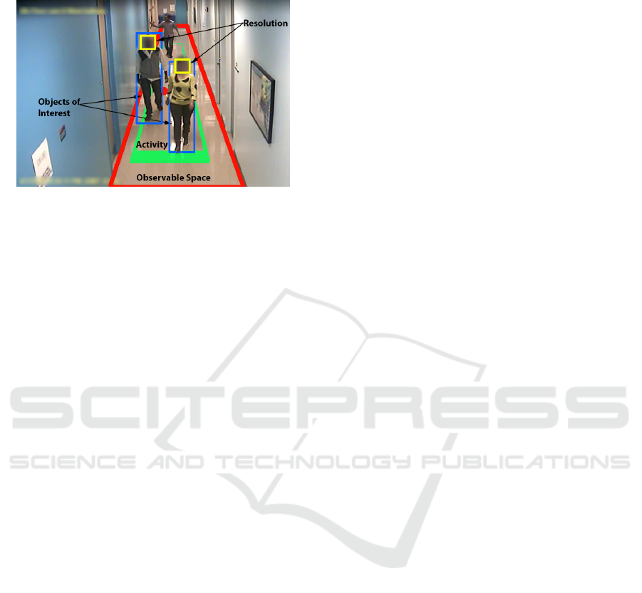
Figure 1: Example of an image from a single surveillance
camera illustrating the four aspects of a camera view.
• the observable space,
• the view of regions within the infrastructure where
dominant activity is expected,
• the ability to capture the preferred pose of objects
of interest (e.g., frontal pose of humans), and
• their image resolution (e.g., face).
Consider a view from a single camera as shown in
Figure 1. In the following, we discuss the four rele-
vant aspects considered for an optimal camera config-
uration.
Maximize Observable Space in View: The in-
formation regarding the 3D geometry (floor) of the
infrastructure can be used to maximize the observable
space. In doing so, only the space that would be ac-
cessible by humans is considered relevant, as depicted
by the red bounding box in Figure 1.
Maximize the View of Regions with Expected
Dominant Human Activity: Given the observable
space, there are regions within it where one can ex-
pect dominant human activity to occur. This is illus-
trated by the green bounding box in Figure 1. All
public infrastructures have entrances, exits and points
of interest. Any doorway can be considered as an en-
trance or an exit. For simplicity they are referred to
as nodes. In an infrastructure, different nodes are ac-
cessed with different frequencies. A node represent-
ing a common entrance or an exit has a high frequency
of access as opposed to an employee’s personal office.
Given these nodes and their probabilities, human mo-
tion can be estimated or measured between the nodes
to identify regions of high human activity.
Maximizes the Ability to Capture Preferred
Pose of Objects of Interest: In this surveillance sce-
nario, frontal pose of the humans can be considered to
be the preferred pose as illustrated by the blue bound-
ing boxes in Figure 1. The direction of motion of
humans can be used to maximize the view of their
frontal pose. Given the nodes, their probabilities, and
trajectories followed by humans, this direction of mo-
tion can be identified.
Resolution of the Imaged Objects: The resolu-
tion of the face (yellow bounding box in Figure 1)
could be considered as a feature of interest in the do-
main of human surveillance, and hence it’s captured
image resolution would be expected to be high. Sim-
ilar to the previous step, the trajectories provide the
direction of motion for the humans. A location of a
face can be assumed based on the estimate of the av-
erage human height. The number of rendered pixels
of the bounding box representing the face in the im-
age from the camera can be used for maximizing this
quantity.
In this paper, we provide a solution for optimal
placement of cameras while considering the above
factors. The main contributions of the paper are:
• We propose a method to incorporate predicted hu-
man behavior for camera placement optimization.
• We propose a method to estimate the human activ-
ity based on the 3D geometry of the infrastructure.
• We propose a method to identify and cluster re-
gions of plausible high human activity.
• We propose a metric to assess the quality of a
camera configuration based on observable space,
amount of activity in the view, preferred pose of
objects of interest, and their image resolution.
2 PREVIOUS WORK
Camera placement optimization is a crucial problem
in computer vision and has been explored by many
researchers. Most of the early work puts empha-
sis on image resolution and were based on a single
camera focused on a static object. The problem was
to find the best position for the camera that maxi-
mizes the quality of features on an object (Tarabanis
et al., 1995; Fleishman et al., 1999). Later, (Chen
and Davis, 2000) proposed a metric based on resolu-
tion and occlusion characteristics of the object that as-
sessed the quality of multiple camera configurations.
The configuration was optimized based on this metric
such that minimum occlusion would occur while en-
suring a certain resolution. (Mittal and Davis, 2004)
suggested a probabilistic approach for visibility anal-
ysis that captured the observable space aspect and cal-
culated the probability of visibility of an object from
at least one camera in the configuration. Then a cost
function was defined that mapped the sensor parame-
VISAPP 2016 - International Conference on Computer Vision Theory and Applications
228

ters to the probability and the cost function was mini-
mized by simulated annealing.
(Erdem and Sclaroff, 2004) suggested a bi-
nary optimization approach for the camera placement
problem that captured both the observable space and
resolution aspect. The polygon representing the space
is fragmented into an occupancy grid and the algo-
rithm tries to minimize the cost of a camera configura-
tion while maintaining some specified spatial resolu-
tion. (H
¨
orster and Lienhart, 2006a; H
¨
orster and Lien-
hart, 2006b; H
¨
orster and Lienhart, 2006c) proposed
a linear programming approach that determines the
calibration for each camera in the network that max-
imizes the coverage of the observable space with a
certain resolution. (Ram et al., 2006; Sivaram et al.,
2009) proposed a performance metric that evaluates
the probability of accomplishing a task as a function
of set of camera configurations. This metric took into
consideration the objects of interest in the scenario
and was defined to realize only images obtained in a
certain direction (frontal image of the person). (Bodor
et al., 2007) proposed a method, where the goal is to
maximize the aggregate observable space across mul-
tiple cameras. An objective function that quantifies
the resolution of the image and the motion trajectories
of the object in the scene is defined. A variant of hill
climbing method was used to maximize this objective
function.
(Murray et al., 2007) applied coverage optimiza-
tion combined with visibility analysis to address this
problem. For each camera location, the coverage was
calculated using visibility analysis. Maximal cov-
ering location problem (MCLP) and backup cover-
age location problem (BCLP) were used to model the
optimum camera combinations and locations. (Ma-
lik and Bajcsy, 2008) suggested a method for opti-
mizing the placement of multiple stereo cameras for
3D reconstruction. An optimization framework was
defined using an error based objective function that
quantifies the stereo localization error along with res-
olution constraints. A genetic algorithm was used to
generate a preliminary solution and later refined us-
ing gradient descent. (Kim and Murray, 2008) also
employed BCLP to solve the camera coverage prob-
lem. They suggested an enhanced representation of
the coverage area by representing it as a continu-
ous variable in contrast to a commonly used discrete
variable. (Yabuta and Kitazawa, 2008) and (Debaque
et al., 2009) also employed a combination of MCLP
and BCLP for solving the optimum camera cover-
age problem. The former took into consideration the
3D geometry of the environment and supplemented
the MCLP/BCLP problem by including a minimal
localization error variable for both monoscopic and
stereoscopic cameras. The optimization problem was
solved using simulated annealing. In the latter, the
MCLP/BCLP problem was supplemented using visi-
bility analysis for optimization. (Huang et al., 2014)
proposed a 2 stage approximation algorithm, the first
part proposes a solution for the minimum watch-
men tour problem and placed cameras along the es-
timated tour, the second part finds the solution to art
gallery problem and added extra cameras to connect
the guards. Most of the previous work emphasizes
the importance of maximizing observable space and
resolution of this space. There is little work address-
ing the significance of activity in the observable space
along with obtaining useful data. This work address
this by assumes equal importance to all four aspects
which were ignored in the previous work.
Considering the 3D geometry of the environment
is of significant value for the camera coverage opti-
mization problem. In this paper, we focus on indoor
scenarios and assume the availability of a complete
3D model of the environment where the camera net-
work is to be deployed. To the best of our knowledge,
this is the first work that takes into consideration the
human activity in the scenario for designing an opti-
mal camera network in the absence of any observa-
tions. Although (Bodor et al., 2007; Janoos et al.,
2007) proposed the use of observed human activity
for optimizing the camera placement, in the proposed
work the human trajectories are simulated and not ob-
served in order to identify regions with dominant hu-
man activity. Furthermore, (Ram et al., 2006; Sivaram
et al., 2009) proposed the use of frontal view from ob-
servations as a task for optimizing the camera position
unlike the proposed method that predicts frontal view
based on human behavior. Finally, the human behav-
ior in a given scenario is influenced by the 3D ge-
ometry of that environment (Mantini and Shah, 2014;
Kitani et al., 2012). To the best of our knowledge,
this is the first work that incorporates this information
to optimize the camera network locations for video
surveillance.
3 METHODOLOGY
3.1 Problem Formulation
Let G be the geometry (floors, ceilings, walls, etc.)
of an infrastructure. Let {C
1
,C
2
,...,C
ν
} be a set
of cameras located in G with configurations (like
position, orientation, zoom, etc.) represented by
{ω
1
,ω
2
,...,ω
ν
},ω
i
∈ Ω, where Ω is the set of all pos-
sible configurations within G. Let g : ω 7→ R be an
objective function. The problem is to find a set of op-
Camera Placement Optimization Conditioned on Human Behavior and 3D Geometry
229

timal configurations {ω
∗
1
,ω
∗
2
,...,ω
∗
ν
} such that:
{ω
∗
1
,ω
∗
2
,...,ω
∗
ν
} = argmax
{ω
1
,ω
2
,...,ω
ν
}∈Ω
ν
∑
i=1
g(ω
i
) (1)
3.2 Camera Coverage Quality Metric
The function g(.) quantifies the following aspects in
view of the camera:
• amount of observable space,
• amount of view of regions with expected domi-
nant activity,
• amount of ability to capture the preferred pose of
objects, and
• image resolution of these objects.
(Janoos et al., 2007) proposed cell coverage qual-
ity metric to determine the coverage quality of a cell
given a set of camera configurations by modeling
realistic camera characteristics. A cell was defined
as any unit of observable space, like a square in a
grid or a triangle in a triangular mesh. Furthermore,
they proposed a cost function that combines this met-
ric with observed human occupancy for optimization.
We extend this notion and define the Camera Cover-
age Quality Metric (CCQM) to quantify amount of
observable space (A), amount view of regions with
expected dominant activity (H), amount of ability to
capture the preferred pose (F) and image resolution
of these objects (R) for a camera configuration ω. The
Camera Coverage Quality Metric (CCQM) is defined
as:
CCQM(ω) = g(A,H,F, R)
=A(ω) ∗H(ω) ∗ F(ω) ∗ R(ω)
(2)
The optimal configuration of the cameras in G is de-
fined as:
{ω
∗
1
,ω
∗
2
,...,ω
∗
ν
} = argmax
{ω
1
,ω
2
,...,ω
ν
}∈Ω
ν
∑
i=1
CCQM(ω
i
) (3)
Given ω, the functions {A,H,F, R} are defined as
follows. Without loss of generality we assume that the
geometry to be viewed is represented by a triangular
mesh containing triangles {t
1
,t
2
,...t
n
} with centroids
{c
1
,c
2
,...c
n
}. Let {t
ω
1
,t
ω
2
,...t
ω
m
} be the set of triangles
in view of the camera with configuration ω.
Amount of Observable Space: The geometric
area in view of the camera is used to quantify this
aspect. The area of coverage function A(ω) is defined
as:
A(ω) =
area
in view
total area
=
∑
m
i=1
area(t
ω
i
)
∑
n
i=1
area(t
i
)
(4)
Amount of View of Regions with Expected
Dominant Activity: An occupancy map of a space
quantifies how often a point is accessed compared to
other points in that space. Let us assume an occu-
pancy map as defined in (Mantini and Shah, 2014),
that defines the frequency with which a triangle is ac-
cessed by humans. The same methodology as fol-
lowed in (Mantini and Shah, 2014) is used to com-
pute the occupancy map. The amount of occupancy is
used to define the activity in the area. If O(t) is the oc-
cupancy of the triangle t, then the human occupancy
volume function is defined as:
H(ω) =
∑
m
i=1
O(t
ω
i
)
∑
n
i=1
O(t
i
)
(5)
Figure 2: Vector discretization of triangle in a triangular
mesh for creating a vector transition histogram from trajec-
tories.
Amount of Ability to Capture the Preferred
Pose of Objects: Humans are considered as objects
of interest. Assuming that τ = {T
1
,T
2
,...} be a set
of trajectories followed by humans in the geometry
G. These trajectories are used to quantify the amount
of frontal view that can be obtained from the con-
figuration ω. For every triangle t
i
in the floor trian-
gular mesh, direction discretization is performed and
eight direction vectors {v
i
1
,v
i
2
,...,v
i
8
} are defined as
by (Zhou et al., 2010)(Figure 2).
In the following step, a vector transition histogram
is constructed from the set of these trajectories. Con-
secutive points in the trajectory are considered to
create a direction vector. If T = {p
1
, p
2
,..., p
l
} is
a trajectory of length l, for all set of consecutive
points {p
i−1
, p
i
}, the direction vector is defined as
(p
i
− p
i−1
). The bin corresponding to the triangle t
in which the point p
i−1
is located and the discretized
direction vector subtending the smallest angle with
(p
i
− p
i−1
) is incremented. Let Ψ(t,v) 7→ R where
t ∈ {t
1
,t
2
,...,t
n
} and v ∈ {v
1
,v
2
,...,v
8
} be the his-
togram function, then the frontal pose function F(ω)
VISAPP 2016 - International Conference on Computer Vision Theory and Applications
230

for a camera with center C is defined as:
F(ω) =
1
m
m
∑
i=1
(((C − c
i
) · v
k−1
)Ψ(t
i
,v
k−1
)
+((C − c
i
) · v
k
)Ψ(t
i
,v
k
)
+((C − c
i
) · v
k+1
)Ψ(t
i
,v
k+1
))
(6)
k = argmax
k
(v
k
· (C − c
i
)) (7)
where t
i
is the triangle with centroid c
i
and v
k
is the
direction vector that subtends the smallest angle with
(C − c
i
).
Image Resolution of the Object: This compo-
nent of CCQM quantifies the resolution of the face.
If the obtained image is far from the camera, the ob-
tained resolution is very low and the image might not
add any value to the system. This component is appli-
cation dependent, it could be customized to obtain a
sufficient resolution of any object, which could be just
the face or the entire body of a human. We follow the
methodology described by (Janoos et al., 2007) and
define the function R(ω) for a camera with center C
as:
R(ω) =
1
m
m
∑
i=1
ρ
ω
(t
i
)
ρ
min
(8)
Algorithm 1: Optimal Pair.
Require: v
1
(ceiling point), L (floor points list)
Ensure: v
2
(Optimal floor point)
1: procedure OPTIMAL–PAIR
2: //Random Search
3: n ← number of points for random search
4: currentv
2
← Random Solution(L)
5: current ← CCQM(v
1
,currentv
2
)
6: for (i = 1; i ≤ n; i + +) do
7: currentv
2
← Random Solution(L)
8: candidate ← CCQM(v
1
,currentv
2
)
9: if candidate > current then
10: current ← candidate
11: candidatev
2
← currentv
2
12: end if
13: end for
14: //Hill Climbing
15: current ← CCQM(v
1
,candidatev
2
)
16: for k ∈ neighbors(candidatev
2
) do
17: currentv
2
← candidatev
2
.neighbor[k]
18: candidate ← CCQM(v
1
,currentv
2
)
19: if candidate > current then
20: current ← candidate
21: v
2
← currentv
2
22: end if
23: end for
24: Return(v
2
)
25: end procedure
ρ
ω
(t
i
) = (2π ∗ d(C,c
i
)
2
(1 − cos(γ/2)))
−1
(σ
k−1
(C − c
i
) · v
k−1
+σ
k
(C − c
i
) · v
k
+σ
k+1
(C − c
i
) · v
k+1
)
(9)
where γ is the Y-field of view defined for the camera,
d(p
1
, p
2
) is the Euclidean distance between the points
p
1
and p
2
, k is as defined in Equation 7, σ is the num-
ber pixels the object occupies in the image and ρ
min
is the user defined value that defines a minimum re-
quired resolution of an object in pixels/inch.
3.3 Optimization
Now that a metric is defined to assess the quality of
a camera configuration ω, we perform a search in
the geometry G to find the optimum parameter ω
∗
.
Given the geometry and the domain knowledge, the
search is performed to find two points, first on the
Algorithm 2: RRHC Optimization.
Require: C (ceiling points list), F (floor points list)
Ensure: v
1
, v
2
(Optimal pair)
1: procedure RRHC–OPTIMIZATION
2: //Random Search
3: n ← number of points for random search
4: currentv
1
← Random–Solution(C)
5: currentv
2
← Optimal–Pair(currentv
1
)
6: current ← CCQM(currentv
1
,currentv
2
)
7: for (i = 1; i ≤ n; i + +) do
8: candv
1
← Random–Solution(C)
9: candv
2
← Optimal–Pair(candv
1
)
10: candidate ← CCQM(candv
1
,candv
2
)
11: if candidate > current then
12: Maxv
1
← candv
1
13: current ← candidate
14: end if
15: end for
16: //Hill Climbing
17: currentv
1
← Maxv
1
18: currentv
2
← Optimal–Pair(currentv
1
)
19: current ← CCQM(currentv
1
,currentv
2
)
20: for k ∈ neighbors(currentv
1
) do
21: candv
1
← currentv
1
.neighbor(k)
22: candv
2
← Optimal–Pair(candv
1
)
23: candidate ← CCQM(candv
1
,candv
2
)
24: if candidate > current then
25: current ← candidate
26: v
1
← candv
1
27: v
2
← candv
2
28: end if
29: end for
30: Return(v
1
,v
2
)
31: end procedure
Camera Placement Optimization Conditioned on Human Behavior and 3D Geometry
231
ceiling to position the camera and the second on the
floor to point the camera towards. Hence the param-
eter ω contains a pair of 3D points {v
1
,v
2
}. A varia-
tion of the hill climbing algorithm called the random-
restart hill climbing (RRHC) algorithm is used for
finding the optimum parameter ω
∗
. Random-restart
hill climbing is an optimization search that provides
near optimal performance (Zhang et al., 2014; Filho
et al., 2010). The idea is to search a limited number
of points randomly and choose the best start location
for hill climbing optimization. Since the objective is
to find two points, one on the floor and the second on
the ceiling, this is done at two levels.
Optimal Pair: This algorithm takes as input a
point on the ceiling (v
1
) along with the list of points
on the floor as input and performs RRHC optimiza-
tion to find the optimal pair v
2
(a point on the floor)
for v
1
that maximizes CCQM (Algorithm 1).
RRHC Optimization: This algorithm takes as in-
put a list of points representing the ceiling (C) and
another list representing the points on the floor (F)
and performs RRHC to find the optimal parameters
{v
1
,v
2
} that maximizes CCQM for a camera, where
v
1
is a point to position the camera and v
2
is a point
for orienting the camera towards (Algorithm 2).
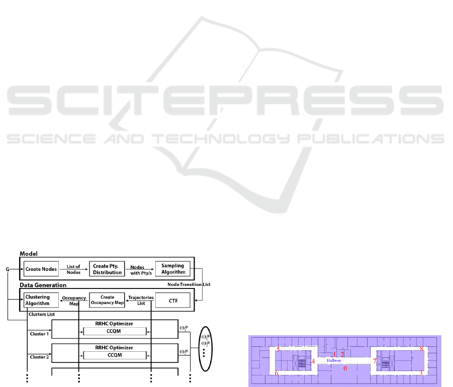
3.4 Framework
The framework for obtaining the optimal parameters
{ω
∗
1
,ω
∗
2
,...,ω
∗
ν
} given the geometry G is described in
this section. The framework design is shown in Fig-
ure 3, which contains three modules.
1. Model: In this module, the infrastructure is mod-
eled. This requires domain knowledge regard-
ing the infrastructure such as entrances, exits and
doors (nodes). Furthermore, knowledge regarding
the frequency of accessing these nodes is also re-
quired. The output is a list of transitions between
Figure 3: Framework with three modules, model, data gen-
eration, and RRHC optimizer for obtaining the optimal pa-
rameters {ω
∗
1
,ω
∗
2
,..., ω
∗
ν
}.
nodes.
2. Data Generation: In this module, the data re-
quired for optimization is generated. The input
is the list of node transitions from the previous
module. First a list of trajectories are generated
using CTF for each pair of nodes from the list.
These are the list of trajectories described in sec-
tion 3.2 for quantifying the amount of preferred
pose of objects of interest. These trajectories are
then given as input to a sub-module that accumu-
lates the trajectories to create an occupancy map
that describes the frequency with which humans
access the geometry. This occupancy map is the
function O(t) described in section 3.2 for quan-
tifying the amount of view of regions with dom-
inant activity. Then the occupancy map is also
input to a clustering algorithm to cluster points
based on their occupancy and spacial location in
the geometry.
3. RRHC Optimizer: Each one of these clusters
obtained is given as input to optimizers for find-
ing the optimized configuration {ω
∗
1
,ω
∗
2
,...,ω
∗
ν
}
for each cluster.
4 EXPERIMENTS
4.1 Implementation
4.1.1 Model
Given the geometry of an infrastructure, most humans
follow trajectories with a goal of reaching a destina-
tion like an entrance, exit or a doorway. There is a cer-
tain probability associated with accessing these nodes
based on the purpose they serve in the infrastructure.
For example at an airport, passengers might access the
ticket counter with a higher probability than a coffee
shop or a restroom. The knowledge of this probability
can be used to sample nodes that humans can transi-
tion between. Let us consider the following test case
scenario. In Figure 4, the objective was to install a
network of cameras that provide effective surveillance
in the hallway.
Figure 4: Floor plan of the test case scenario where the cam-
eras are to be placed. The nodes are labeled with numbers.
VISAPP 2016 - International Conference on Computer Vision Theory and Applications
232

Create Nodes and Probability Distribution:
The identified nodes are labeled with numbers in Fig-
ure 4. Let {n
1
,n
2
,...} be the nodes in the geometry
G. In the absence of any observations of human mo-
tion, the probability of accessing a node was assumed
to be proportional to the accommodation capacity of
the room unless it was an entrance or exit. Implying
that higher the capacity of a room to hold/seat peo-
ple, the higher was the probability of accessing it. If
P
a
(n
i
) is a probability function that assigns probabil-
ity to a node n
i
and A
c
(n
i
) is its accommodation ca-
pacity, then
P
a
(n
i
) ∝
0 if n
i
= entry/exit
A
c
(n
i
) otherwise
(10)
Sampling Algorithm: The sampling algorithm
was designed based on few assumption. A human en-
tering the geometry G would eventually exit. A hu-
man would access a minimum of one node before ex-
iting the geometry. Algorithm 3 describes the steps.
Algorithm 3: Nodes Sampling.
1: Choose a random entrance
2: Choose a node to access using P
a
as distribution
3: Choose randomly to either exit or access another
node
4: if access another node then
5: Choose another node excluding the current
node
6: Goto step 3
7: else
8: Choose a random exit
9: end if
In the example geometry in Figure 4, an en-
try (4, 7) was chosen with equal probability, then a
node was chosen that is not an exit based on the as-
signed probability (P
a
). Now assuming that the hu-
man had transitioned to the node, the human could ei-
ther choose to transition to another node or exit with
equal probability. If the human chose to exit, the clos-
est exit was chosen, else the human would choose to
go to another node based on a calculated probability.
The probability of choosing the second node changed
because the node that the human was currently in was
eliminated when calculating the probabilities. This
gave a list of nodes {n
s
1
,n
s
2
,...} that can be used as
start and end nodes for simulating trajectories.
4.1.2 Data Generation
Given the geometry of the environment along with
the nodes and their assigned probabilities, the likely
Figure 5: Occupancy map (O(t)) of the hallway obtained
by mapping multiple simulated trajectories. Red indicating
regions of dominant activity and blue with minor activity.
human motion in the infrastructure was simulated to
identify regions of dominant human activity.
Contextual Trajectory Forecasting (CTF):
CTF (Mantini and Shah, 2014) was used to simulate
trajectories from the start node to the end node.
Given the 3D geometry of the environment and the
starting point and destination of a human, CTF is
assembled on two assumptions. First, the human
would follow a path that requires the shortest time
to reach the destination, and second, the human
would adhere to certain behavioral norms that are
observed when walking in hallways. CTF uses a
Markov model and assigns probabilities to points on
the floor such that consecutive points are sampled
from start to destination to form a trajectory that
represents the shortest path while conforming to
observed behavioral norms. CTF can take any pair of
nodes {n
s
i
,n
s
j
} from the previous step and produce a
trajectory T
s
i j
= {n
s
i
, p
s
1
, p
s
2
,....,n
s
j
}.
Create Occupancy Map (O(t)): In this step,
multiple pairs of nodes were generated as described in
the previous step. These generated nodes were input
to CTF to obtain a set of trajectories τ = {T
1
,T
2
,...,}.
These are the set of trajectories used for quantifying
the preferred pose of objects of interest as described
in section 3.2. These trajectories were mapped to
the floor in the geometry to create an occupancy map
O(t
i
) which quantifies the number of times a trajec-
tory passes through a triangle t
i
as used in quantifying
the amount of view of regions with dominant activity
in section 3.2. A snapshot of the occupancy map from
the simulated trajectories T in G is shown in Figure 5.
Clustering Algorithm: The regions that belong
to the same cluster should have a similar value of oc-
cupancy and also be located in the same spacial loca-
tion. A point’s spatial co-ordinates and it’s occupancy
(c
i
,O(t
i
)) were used as features, where c
i
= {x
i
,y
i
,z
i
}
are the 3D co-ordinates of the centroid of triangle t
i
and O(t
i
) it’s occupancy. The clusters obtained by us-
ing Expectation Maximization (EM) (Dempster et al.,
Figure 6: Clusters of regions with dominant activity in the
geometry obtained by EM algorithm.
Camera Placement Optimization Conditioned on Human Behavior and 3D Geometry
233
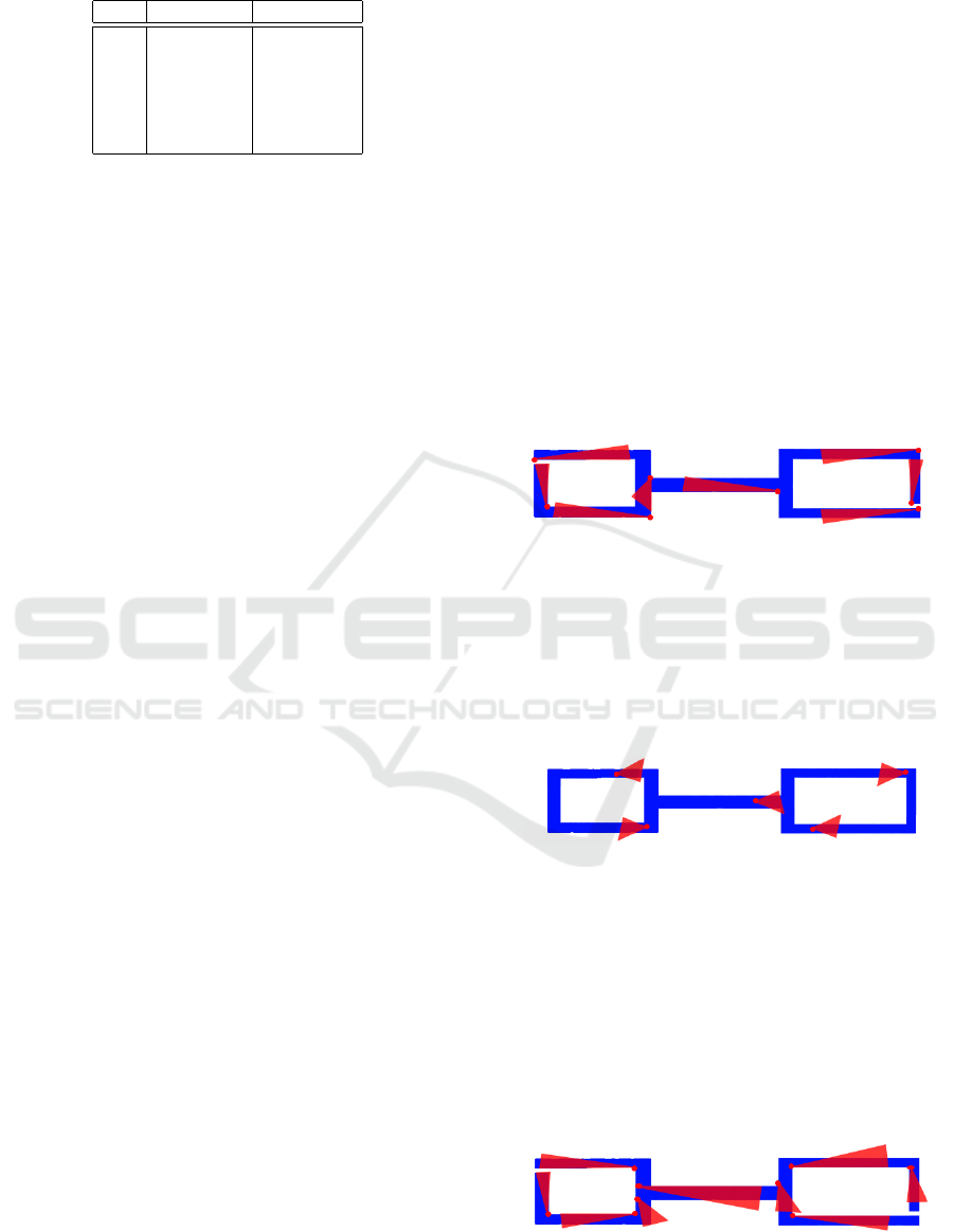
Table 1: Identified clusters and their mean occupancies.
No. Cluster Occupancy
1 Blue 0.23
2 Red 0.42
3 Green 0.13
4 Aqua 0.11
5 Light Pink 0
6 Pink 0.11
1977) are shown in Figure 6. In this scenario, red
cluster was identified to have the highest average hu-
man occupancy followed by blue and then pink as
shown in Table 1.
4.1.3 RRHC Optimization
Once the clusters are identified, the optimization is
applied on each cluster separately. Given a cluster,
first the points in the ceiling that have a view of the
centroid of the cluster are identified and these points
are considered as the possible location of the cameras.
The only possible orientation for a camera are point-
ing towards the points on the floor in the cluster. This
would simplify the problem to finding two points, one
on the ceiling to position the camera and the second
on the floor to point the camera towards. As described
in section 3.3, random restart hill climbing optimiza-
tion was performed to find the two optimal points.
4.2 Results
The motivation for this work was to optimize the cam-
era placement in the geometry to provide effective
surveillance as defined in section 1. A configuration
of cameras in a geometry is considered to provide ef-
fective surveillance if it maximizes the below quanti-
ties while minimizing the number of cameras. Such a
system is effective both in terms of surveillance and
cost. Hence all the quantities used for comparison are
normalized by the number of cameras in the configu-
ration.
• Area of Observable Space in View: The total
area accessible by humans in view of the camera
is calculated for all the cameras and normalized.
• Amount of Activity in View: To quantify the oc-
cupancy of a location that is in view, the activity
produced in that location is considered. The num-
ber of frames that have motion in them are used as
a metric to define the activity of the location that
is viewed from the camera. The normalized value
is used as a metric.
• Pose of Objects of Interest and their Resolu-
tion: Assuming that a certain number of pixels are
required for face detection. Face detection is used
to quantify the pose of objects of interest along
with their resolution. The number of faces de-
tected are counted for every camera in the con-
figuration and normalized.
The above metrics are defined to assess these quali-
ties in a configuration of cameras. The configuration
generated by the proposed method is compared to the
following method.
• 3 Coloring Solution (Fisk, 1978): A solution
to Art Gallery Problem (AGP) was obtained us-
ing the 3 coloring solution and the cameras were
placed at these locations. This configuration was
used as baseline. The geometry of the environ-
ment’s polygon contains holes. The polygon was
modified to remove the holes and then 3 coloring
solution was computed for the polygon. The cam-
eras were manually placed to maximize the area
in view. The solution is as shown in Figure 7.
Figure 7: Configuration of cameras obtained by computing
3 coloring solution to AGP.
• (Janoos et al., 2007): Janoos et al. defined cell
coverage quality metric by taking observed hu-
man occupancy and resolution into account. This
metric was used to optimize the camera location
for each cluster. The following configuration was
obtained, see Figure 8.
Figure 8: Configuration of cameras obtained by optimizing
the cell coverage quality metric proposed bt Janoos et al.
2007 for each cluster.(Janoos et al., 2007).
• (Huang et al., 2014): Huang et al. proposed a
shortest watchman route solution and positioned
wireless cameras along the route to maximize the
view area of the polygon. Their solution was pro-
posed only for simple polygons with out holes and
hence the modified polygon was used in this case
as well. The obtained configuration is shown in
Figure 9.
Figure 9: Configuration of cameras obtained by finding the
shortest watchman route in the geometry as proposed by
Huang et al. 2014(Huang et al., 2014).
VISAPP 2016 - International Conference on Computer Vision Theory and Applications
234

Figure 10: Configuration of cameras obtained from the pro-
posed method.
• Proposed Method: The obtained configuration
from the proposed method is shown in Figure 10,
and the view from the cameras are shown in Fig-
ure 11.
Cam. 1 Cam. 2
Cam. 3 Cam. 4
Cam. 5
Figure 11: Camera view from the cameras deployed in the
test case scenario as calculated by the proposed method.
Table 2 shows the area under view per camera.
Although, 3 coloring solution and Huang et al. has
higher area coverage, the number of cameras used is
higher than that of the proposed method and the area
in view per camera is higher for the proposed method.
Table 2: Comparison of area and activity in view per cam-
era.
Method no. of cams. Area/cam Activity/cam
3 Coloring 8 0.057 28048.6
Janoos 5 0.01 44366.2
Huang 10 0.064 40092.5
Proposed 5 0.109 69933.8
All cameras used for experiments had a frame rate
of 30fps. For each camera, the number of frames in
which there is activity is counted using background
subtraction. The average number of frames per cam-
era are shown in Table 2. Most activity per camera
was observed in the proposed method.
For each of these methods, a day’s worth of data
(10 hours) was collected. We have run face detec-
tion (Viola and Jones, 2001; Lienhart and Maydt,
2002) on these videos to count the number of faces
Table 3: Faces counted from individual cameras in the pro-
posed method.
Camera Faces
Cam. 1 622
Cam. 2 3430
Cam. 3 5929
Cam. 4 915
Cam. 5 1930
captured. The number of faces captured for each cam-
era are shown in Table 3. It can be noticed that Cam.
3 has the highest number of faces detected followed
by Cam. 2. Cam. 3 is over-viewing the common
hallway represented by the red cluster (see Table 1)
with the highest simulated occupancy value. The av-
erage number of faces detected for each method are
shown in Table 4. Approximately the same total num-
ber of faces were detected by 3 coloring solution and
the proposed method, except for 3 coloring solution
uses 8 cameras and the proposed method uses only 5
cameras. Using Huang et al. more than twice the to-
tal number of faces were detected than the proposed
method but the number of cameras used were also
twice as many than the proposed method. More than
a quarter of the faces detected by Huang et al. con-
figuration were from a single camera of the 10 cam-
eras, which coincidentally happened to be focused at
an elevator where people tend to stand and wait. The
method proposed by Janoos et al. focuses on areas
with high human occupancy and takes resolution of
the triangle into account as opposed to the proposed
method which uses the resolution of the approximate
location of the face and hence their cameras are lo-
cated above the regions of dominant human occu-
pancy and fails to capture faces.
Table 4: Comparison of faces detected per camera.
Method cameras Faces/cam
3 Coloring 8 1264
Janoos 5 1111.8
Huang 10 2040.5
Proposed 5 2183.6
Although the proposed system performs better
over the state of the art systems, some necessary im-
provements are to be taken into consideration. As no-
ticed in Huang et al. configuration, significant num-
ber of faces were captured by focusing a camera at
the elevator. This can be considered as a draw back
of the proposed system and all the others being com-
pared to, as none of the systems take the entrances
and exits into consideration which could be valuable
for surveillance. It would be interesting to incorpo-
rate a method to include the entrances and exits in the
Camera Placement Optimization Conditioned on Human Behavior and 3D Geometry
235

analysis. A method to estimate the number of cam-
eras required for each cluster depending on the size
of the cluster can be useful. If the cluster is big, it
might be interesting to assign multiple cameras and
incorporate a MCLP/BCLP problem formulation for
optimization to ensure maximal coverage.
5 CONCLUSION
We have proposed an algorithm to optimize the place-
ment of surveillance cameras in a 3D infrastructure
by predicting the possible human behavior within the
infrastructure. We have proposed a method to iden-
tify regions with dominant human activity. We have
also proposed a metric that quantifies the position of a
camera based on the observable space, activity in this
space, pose of objects of interest within the activity
and their image resolution in camera view for opti-
mization. This method was compared with the state
of the art algorithms and the obtained results show an
improvement in the amount of area under view, ob-
served activity and face detection rate per camera.
ACKNOWLEDGEMENT
This work was supported in part by the US Depart-
ment of Justice 2009-MU-MU-K004. Any opinions,
findings, conclusions or recommendations expressed
in this paper are those of the authors and do not nec-
essarily reflect the views of our sponsors.
REFERENCES
Bodor, R., Drenner, A., Schrater, P., and Papanikolopoulos,
N. (2007). Optimal camera placement for automated
surveillance tasks. Journal of Intelligent and Robotic
Systems, 50(3):257–295.
Chen, X. and Davis, J. (2000). Camera placement consid-
ering occlusion for robust motion capture. Technical
report.
Debaque, B., Jedidi, R., and Prevost, D. (2009). Optimal
video camera network deployment to support security
monitoring. In Information Fusion, 2009. FUSION
’09. 12th International Conference on, pages 1730–
1736.
Dempster, A. P., Laird, N. M., and Rubin, D. B. (1977).
Maximum likelihood from incomplete data via the em
algorithm. JOURNAL OF THE ROYAL STATISTICAL
SOCIETY, SERIES B, 39(1):1–38.
Erdem, U. M. and Sclaroff, S. (2004). Optimal placement of
cameras in floorplans to satisfy task requirements and
cost constraints. In In Proc. of OMNIVIS Workshop.
Filho, C., de Oliveira, A., and Costa, M. (2010). Us-
ing random restart hill climbing algorithm for mini-
mization of component assembly time printed circuit
boards. Latin America Transactions, IEEE (Revista
IEEE America Latina), 8(1):23–29.
Fisk, S. (1978). A short proof of Chvtal’s Watchman Theo-
rem. Journal of Combinatorial Theory, 24.
Fleishman, S., Cohen-Or, D., and Lischinski, D. (1999).
Automatic camera placement for image-based model-
ing. In Computer Graphics and Applications, 1999.
Proceedings. Seventh Pacific Conference on, pages
12–20, 315.
H
¨
orster, E. and Lienhart, R. (2006a). Approximating opti-
mal visual sensor placement. In Multimedia and Expo,
2006 IEEE International Conference on, pages 1257–
1260.
H
¨
orster, E. and Lienhart, R. (2006b). Calibrating and op-
timizing poses of visual sensors in distributed plat-
forms. Multimedia Systems, 12(3):195–210.
H
¨
orster, E. and Lienhart, R. (2006c). On the optimal place-
ment of multiple visual sensors. In Proceedings of the
4th ACM International Workshop on Video Surveil-
lance and Sensor Networks, VSSN ’06, pages 111–
120, New York, NY, USA. ACM.
Huang, H., Ni, C.-C., Ban, X., Gao, J., Schneider, A., and
Lin, S. (2014). Connected wireless camera network
deployment with visibility coverage. In INFOCOM,
2014 Proceedings IEEE.
Janoos, F., Machiraju, R., Parent, R., Davis, J. W., and Mur-
ray, A. (2007). Sensor configuration for coverage opti-
mization for surveillance applications. In SPIE, 2007
Proceedings.
Kim, K. and Murray, A. T. (2008). Enhancing spatial repre-
sentation in primary and secondary coverage location
modeling*. Journal of Regional Science, 48(4):745–
768.
Kitani, K., Ziebart, B., Bagnell, J., and Hebert, M. (2012).
Activity forecasting. Lecture Notes in Computer Sci-
ence, pages 201–214.
Lienhart, R. and Maydt, J. (2002). An extended set of haar-
like features for rapid object detection. In Image Pro-
cessing. 2002. Proceedings. 2002 International Con-
ference on, volume 1, pages I–900–I–903 vol.1.
Malik, R. and Bajcsy, P. (2008). Automated Placement of
Multiple Stereo Cameras. In The 8th Workshop on
Omnidirectional Vision, Camera Networks and Non-
classical Cameras - OMNIVIS, Marseille, France.
Rahul Swaminathan and Vincenzo Caglioti and An-
tonis Argyros.
Mantini, P. and Shah, S. (2014). Human trajectory fore-
casting in indoor environments using geometric con-
text. In Proceedings of the Ninth Indian Conference
on Computer Vision, Graphics and Image Processing,
ICVGIP ’14. ACM.
Mittal, A. and Davis, L. (2004). Visibility analysis and sen-
sor planning in dynamic environments. In Pajdla, T.
and Matas, J., editors, Computer Vision - ECCV 2004,
volume 3021 of Lecture Notes in Computer Science,
pages 175–189. Springer Berlin Heidelberg.
VISAPP 2016 - International Conference on Computer Vision Theory and Applications
236

Murray, A. T., Kim, K., Davis, J. W., Machiraju, R., and
Parent, R. (2007). Coverage optimization to support
security monitoring. Computers, Environment and
Urban Systems, 31(2):133 – 147.
Ram, S., Ramakrishnan, K. R., Atrey, P. K., Singh, V. K.,
and Kankanhalli, M. S. (2006). A design methodol-
ogy for selection and placement of sensors in mul-
timedia surveillance systems. In Proceedings of the
4th ACM International Workshop on Video Surveil-
lance and Sensor Networks, VSSN ’06, pages 121–
130, New York, NY, USA. ACM.
Sivaram, G. S. V. S., Kankanhalli, M. S., and Ramakrish-
nan, K. R. (2009). Design of multimedia surveillance
systems. ACM Trans. Multimedia Comput. Commun.
Appl., 5(3):23:1–23:25.
Tarabanis, K., Allen, P., and Tsai, R. (1995). A survey of
sensor planning in computer vision. Robotics and Au-
tomation, IEEE Transactions on, 11(1):86–104.
Viola, P. and Jones, M. (2001). Rapid object detection using
a boosted cascade of simple features. In Computer Vi-
sion and Pattern Recognition, 2001. CVPR 2001. Pro-
ceedings of the 2001 IEEE Computer Society Confer-
ence on, volume 1, pages I–511–I–518 vol.1.
Yabuta, K. and Kitazawa, H. (2008). Optimum camera
placement considering camera specification for secu-
rity monitoring. In Circuits and Systems, 2008. ISCAS
2008. IEEE International Symposium on, pages 2114–
2117.
Zhang, Y., Lei, T., Barzilay, R., and Jaakkola, T. (2014).
Greed is Good if Randomized: New Inference for De-
pendency Parsing. In Proceedings of the 2014 Con-
ference on Empirical Methods in Natural Language
Processing (EMNLP). Association for Computational
Linguistics.
Zhou, W., Xiong, H., Ge, Y., Yu, J., Ozdemir, H., and
Lee, K. (2010). Direction clustering for characteriz-
ing movement patterns. In Information Reuse and In-
tegration (IRI), 2010 IEEE International Conference
on, pages 165–170.
Camera Placement Optimization Conditioned on Human Behavior and 3D Geometry
237
