
Neural Network based Novelty Detection for Incremental
Semi-supervised Learning in Multi-class Gesture Recognition
Husam Al-Behadili
1,2
, Arne Grumpe
2
and Christian W
¨
ohler
2
1
Electrical Engineering, University of Mustansiriyah, Al-Mustansiriyah, Box 46007, Baghdad, Iraq
2
Image Analysis Group, TU Dortmund University, Otto-Hahn-Str. 4, D–44227, Dortmund, Germany
Keywords:
Data Stream, Neural Network, Extreme learning Machine (ELM), Novelty Detection, Incremental Learning,
Semi-supervised Learning, Extreme Value Theory (EVT), Confidence Band.
Abstract:
The problems of infinitely long data streams and its concept drift as well as non-linearly separable classes
and the possible emergence of “novel classes” are topics of high relevance for gesture data streaming based
automatic recognition systems. To address these problems we apply a semi-supervised learning technique
using a neural network in combination with an incremental update rule. Neural networks have been shown
to handle non-linearly separable data and the incremental update ensures that the parameters of the classifier
follow the “concept-drift” without the necessity of an increased training set. Since a semi-supervised learning
technique is sensitive to false labels, we apply an outlier detection method based on extreme value theory and
confidence band intervals. The proposed algorithm uses the extreme learning machine, which is easily updated
and works with multi-classes. A comparison with an auto-encoder neural network shows that the proposed
algorithm has superior properties. Especially, the processing time is greatly reduced.
1 INTRODUCTION
When people start a conversation, they commonly use
hand motions. These motions of the hand may also
be used to communicate with machines in Human-
Machine Interaction (HMI). In this context, they are
called “gestures”. Since gestures are considered an
intuitive, fast and save way in HMI, they are included
in many applications ranging from computer games to
applications in the medical industry (e.g. Yusoff et al.
(2013)). Gestures of the same class, however, may
be performed in a different manner by different per-
sons or by the same individual if she/he performs the
gesture more than once. Hence, the classifier should
be trained with all possible gestures to get an accept-
able recognition rate. Unfortunately, manually la-
belled data are scarce. Unlabelled data, in contrast,
may be streamed continuously. Consequently, semi-
supervised learning may be applied to solve this prob-
lem. Semi-supervised learning corresponds to first
training a classifier on a labelled data set in a super-
vised manner and updating the training set using the
labels assigned by the classifier itself (Zhu and Gold-
berg, 2009). However, the problems arising from the
usage of streamed data are the “infinite length” and
the “concept-drift”. They were addressed by most of
the existing on-line algorithms (Masud et al., 2011).
In addition, non-linearly separable distributions of the
data, the emersion of new classes or outliers, and the
computational complexity are possible problems. To
address these problems we apply a semi-supervised
learning technique using a neural network in combi-
nation with an incremental update rule. Neural net-
works have been shown to handle non-linearly sep-
arable data and the incremental update ensures that
the parameters of the classifier follow the “concept-
drift” without the necessity of an increased training
set. Since a semi-supervised learning technique is
sensitive to false labels, we apply an outlier detec-
tion method based on the concepts of extreme value
theory and confidence bands interval to suppress false
labels that will potentially affect the performance of
the classifier after the next training cycle.
2 RELATED WORK
There have been several research studies on semi-
supervised learning (Zhu and Goldberg, 2009). The
semi-supervised techniques are categorized in three
main types, which are: First, guessing the unlabelled
data and subsequently retraining the classifier using
Al-Behadili, H., Grumpe, A. and Wöhler, C.
Neural Network based Novelty Detection for Incremental Semi-supervised Learning in Multi-class Gesture Recognition.
DOI: 10.5220/0005674202870294
In Proceedings of the 11th Joint Conference on Computer Vision, Imaging and Computer Graphics Theory and Applications (VISIGRAPP 2016) - Volume 3: VISAPP, pages 289-296
ISBN: 978-989-758-175-5
Copyright
c
2016 by SCITEPRESS – Science and Technology Publications, Lda. All rights reserved
289

these labels, e.g. EM, co-training, and transductive
SVM (Zhu and Goldberg, 2009). Second, finding
additional features derived from the unlabelled data
(Johnson and Zhang, 2015). Third, manifold reg-
ularization has been used to leverage the labelled
and unlabelled data (Huang et al., 2014). Recently,
the extreme learning machine was applied to semi-
supervised learning, since it has favourable features.
Huang et al. (2014) constructed the Laplacian graph
from labelled and unlabelled data to extend the ex-
treme learning machine for semi-supervised learning.
They, however, supposed all unlabelled data to be
available together at the beginning of the training.
Hence, it is not suitable for data streams. A new ap-
proach by Li et al. (2013) applied co-training to train
the ELM in a semi-supervised manner. Since, this al-
gorithm repeatedly trains several ELMs, it is consid-
ered computationally costly. Since neural networks
have the ability to approximate the non-linear map-
ping from features to classes directly from the input
samples, several researchers proposed different algo-
rithms of incremental neural networks. Huang et al.
(2006a) introduced the “incremental extreme learn-
ing machine” (IELM) by adding randomly generated
nodes to a single-layer feed-forward network (SLFN)
and computed the output weight analytically for the
new nodes only. Since semi-supervised learning is
sensitive to false labels, the proposed algorithm needs
to detect and reject the outliers which may affect on
the performance of the algorithm. Pimentel et al.
(2014) describe methods solving the novelty detec-
tion problem by using statistical techniques or neu-
ral networks. Applications of neural networks have
been implemented in many domains (Hugueny et al.,
2009). Due to the large variety of artificial neural
networks many different neural network approaches
may be used for novelty detection. Tax (2001) used
the auto-associative neural networks (AANN) as an
one class classifiers within the data discretion, out-
lier and novelty detection toolbox (ddtools)
1
(Tax,
2015), where the auto-encoder function is called “au-
toenc dd”. It is a reference for our work and is ex-
plained in detail in the next section.
3 REFERENCE METHODS
3.1 Extreme Learning Machine (ELM)
The concept of the ELM is described in detail by
Huang et al. (2006b), whose description we follow
here. According to their approach, for a SLFN with L
1
http://prlab.tudelft.nl/david-tax/dd tools.html
hidden neurons the output is given by
f
l
(~x
j
) =
L
∑
i=1
β
i
G(~a
i
,b
i
,~x
j
) ~x
j
∈ R
n
,~a
i
∈ R
n
(1)
with β
i
as the output weight, ~a
i
and b
i
as the learn-
ing parameters, G(~a
i
,b
i
,~x
j
) as hidden neuron output i,
and ~x
j
as the feature vector associated with training
sample j. It is
G(~a
i
,b
i
,~x
j
) = g(~a
i
·~x
j
+ b
i
), b
i
∈ R (2)
with ~a
i
and b
i
as the ith neuron’s input weight vector
and bias. For hidden neurons with radial basis func-
tion (RBF) characteristic it is,
G(~a
i
,b
i
,~x
j
) = g(b
i
~x
j
−~a
i
) b
i
∈ R
+
(3)
with~a
i
and b
i
as the centre and width of RBF neuron i.
R
+
refers to all positive real numbers (Huang et al.,
2006b).
The ELM is a SLFN network, and the equations
above apply to it. Following Huang et al. (2006b),
suppose we have m arbitrary distinct sample (~x
j
∈ R
n
,
~
t
j
∈ R
c
) consisting of a feature vector ~x
j
and a tar-
get vector
~
t
j
containing one value for each of the c
classes, respectively. Notably, it is
~
t
j
= +1 for the
output neuron belonging to the class of the sample
and
~
t
j
= −1 for the other output neurons, respectively.
The ELM has L neurons. An error-free approximation
of the m samples by this ELM then implies the exis-
tence of a set of parameters β
i
, ~a
i
and b
i
fulfilling
f
L
(~x
j
) = t
j
, j = 1 · · · m, (4)
which can be written as a matrix
H
H
H · β
β
β = T
T
T (5)
H
H
H =
G(~a
1
,b
1
,~x
1
) ··· G(~a
L
,b
L
,~x
1
)
.
.
.
.
.
.
.
.
.
G(~a
1
,b
1
,~x
m
) ··· G(~a
L
,b
L
,~x
m
)
m×L
,
(6)
β
β
β =
~
β
T
1
.
.
.
~
β
T
L
L×c
and T
T
T =
~
t
T
1
.
.
.
~
t
T
m
m×c
(7)
where
~
β
i
denotes the vector containing the ith neu-
ron’s output weight for all classes and the mtrix H
H
H
denotes the hidden layer output. According to Huang
et al. (2006b), the procedure of training the ELM is as
follows:
• The first step is to assign the input parameters (i.e.
~a
i
, and b
i
, i = 1, . . . , L) randomly.
• Analytical computation of the matrix H
H
H is per-
formed according to Eq. (7).
VISAPP 2016 - International Conference on Computer Vision Theory and Applications
290

• The output weights are then estimated using (5).
As shown by Huang et al. (2006b), the problem here
is to minimize the error in (5), i.e.
k
H
H
H · β
β
β − T
T
T
k
. Since
(5) is a linear system in the output weights, the output
weights are estimated by Huang et al. (2006b) using
the pseudoinverse of the output matrix of the hidden
layer according to H
H
H
†
= (H
H
H
T
H
H
H)
−1
H
H
H
T
(Rao and Mi-
tra, 1971):
ˆ
β
β
β = H
H
H
†
· T
T
T (8)
As suggested by Huang et al. (2006b), the singular
value decomposition (SVD) (Rao and Mitra, 1971) is
used to compute the pseudoinverse H
H
H
†
. The labels of
the new samples can then be obtained by using the
estimates
ˆ
β
β
β and H
H
H
†
in (7).
3.2 Extreme Value Theory (EVT)
The conventional approaches of the novelty detec-
tion mostly require one threshold or a set of class-
wise thresholds computed by additional manually la-
belled data or by using the cross-validation process,
which are either need additional labelled data or are
time consuming. In contrast, the extreme value the-
ory (EVT) as described by Roberts (1999) and Clifton
et al. (2008) avoids these problems. It is a statistical
theory used to model the extreme values, i.e. maxima
or minima in the one-dimensional case, in the tails of
the distributions. Following Roberts (1999), let there
be a set of m i.i.d. random samples X =
{
~x
1
,~x
2
...,~x
m
}
each of them is n-dimensional and distributed as given
by the probability density function f (~x). Further-
more, let the extreme value of X be ~x
max
. Given the
set X , the probability of ~x being more extreme than
~x
max
is the extreme value probability which expressed
as P
EV
(~x|X ) = P(~x
x
<~x). There are three types of dis-
tributions of the EVD as stated by the Fisher-Tippett
theorem (Fisher and Tippett, 1928): the Gumbel dis-
tribution, the Frechet distribution and the Weibull dis-
tribution (Roberts, 1999). As described by Roberts
(1999) and Clifton et al. (2008), the Gumbel distri-
bution models the EVD of data originating from the
one-dimensional one-sided normal distribution with
a mean value of zero and a variance of 1, i.e. D =
N (0, 1)
. According to Clifton et al. (2008), the
Gumbel distribution for a one-dimensional variable x
P
Gumbel
(x|X ) = exp
−exp
−
x − µ
m
σ
m
, (9)
is defined by the location parameter
µ
m
= (2 ln(m))
0.5
−
ln(ln(m)) + ln(2π)
2(2ln(m))
0.5
(10)
and the scale parameter
σ
m
= (2 ln(m))
0.5
. (11)
Both parameters depend only on m, i.e. the number
of samples drawn from D. These minimize or absorb
the effect of the amount of training data on the final
results and thus the threshold remains unchanged with
an increasing amount training data.
We define a threshold P
th
that is based on the ex-
treme values of the known classes. A novelty is de-
tected if P
EV
exceeds this threshold. As may be ver-
ified from the equations above, the threshold in EVT
has a direct statistical interpretation and does not de-
pend on the distribution of the classes whereas the
conventional thresholds depend on the distribution of
the classes.
3.3 Auto-associative Neural Networks
Auto-associative neural networks (AANN) or auto-
encoder networks (AutoENC), as they are called by
Tax (2001), are neural networks that learn a data rep-
resentation (Hertz et al., 1991), i.e. an AANN recon-
structs the input pattern at their output layer. In this
work, we apply the auto-encoder from the toolbox
presented by Tax and Duin (1999). In this toolbox the
auto-encoder architecture has only one hidden layer
with h
auto
hidden units. Sigmoid transfer functions
are used for the hidden neurons. It is trained by min-
imizing the mean squared deviation of the input from
the output. The error is used as a measure for the nov-
elty detection. It is supposed that the target patterns
will be reconstructed with smaller errors than outliers.
The error E
AANN
of an input ~x is
E
AANN
=
k
f
AANN
(~x,~w) −~x
k
2
(12)
where f
ANN
is transfer function of the AANN and ~w
is a vector containing its parameters. The problems of
the AANN to novelty detection are the same problems
as those arising from the conventional application of
neural networks to classification problems: It requires
a pre-defined number of neurons, a learning rate, and
stopping criteria from an expert user. In our experi-
ments, the best number of neurons is 5, which is the
default number in the function of the toolbox. We also
used the default outlier percentage 5% that is used to
compute the threshold of the novelty.
3.4 Confidence Bands
Since measurements are affected by noise, models
derived from these measurements differ for each ac-
quired set of new data. The confidence band en-
closes all models obtained from the measurements
with a specified probability (Kardaun, 2005). Con-
fidence bands are computed in several approaches
Neural Network based Novelty Detection for Incremental Semi-supervised Learning in Multi-class Gesture Recognition
291

(e.g. Kendall et al., 2007). In the context of semi-
supervised learning, the confidence bands of a poly-
nomial classifier are used by Al-Behadili et al. (2014)
to detect outlier samples.
4 THE PROPOSED ALGORITHM
Here, we propose a method to update the ELM in-
crementally and to apply the outliers detection using
the EVT and the confidence band to the output of the
ELM to reject the outliers. The proposed algorithm
extends the approach of Al-Behadili et al. (2015),
which uses only EVT for detecting the outliers. It
consists of two phases.
4.1 Incremental Learning Phase
The incremental updating rule is derived based on the
pseudoinverse method introduced by Lan et al. (2009)
according to
M
M
M = H
H
H
T
H
H
H and P
P
P = H
H
H
T
T
T
T . (13)
Hence, β
β
β = M
M
M
−1
P
P
P. (14)
The dimension of M
M
M is L × L and the dimension of
the P
P
P is L × c, where L corresponds to the number of
hidden neurons and c to the number of classes.
Suppose that we have m
(0)
labelled samples for
initial training. We then compute M
M
M
(0)
= H
H
H
T
(0)
H
H
H
(0)
and P
P
P
(0)
= H
H
H
T
(0)
T
T
T
(0)
according to (13). Hence, β
β
β
(0)
=
M
M
M
−1
(0)
P
P
P
(0)
.
Incremental learning is achieved by adding
chunks of samples to the training set. If the number
of samples
~
ˆx in the chunk k + 1 is ˆm then the hidden
layer output matrix
ˆ
H
H
H corresponding to the new chunk
of data is
ˆ
H
H
H =
G(~a
1
,b
1
,
~
ˆx
1
) ··· G(~a
L
,b
L
,
~
ˆx
1
)
.
.
.
.
.
.
.
.
.
G(~a
1
,b
1
,
~
ˆx
ˆm
) ··· G(~a
L
,b
L
,
~
ˆx
ˆm
)
ˆm×L
(15)
From (15) and (13) it follows that
ˆ
M
M
M =
ˆ
H
H
H
T
ˆ
H
H
H and
ˆ
P
P
P =
ˆ
H
H
H
T
ˆ
T
T
T corresponding to the new chunk data. Then
M
M
M
(k+1)
= M
M
M
(k)
+
ˆ
M
M
M and P
P
P
(k+1)
= P
P
P
(k)
+
ˆ
P
P
P (16)
Finally, using (14) the updated output is β
β
β
(k+1)
=
M
M
M
−1
(k+1)
P
P
P
(k+1)
.
4.2 Novelty Detection Phase
4.2.1 Novelty Detection using EVT
According to Huang et al. (2006b), the output of the
ELM is around +1 for the class that the sample be-
longs to it and around −1 for the other classes. This
follows immediately from the target values used for
the training of the ELM. If the output of the winner
class is exactly +1 then this result is similar to the
training data and thus highly believable. The confi-
dence of the result decreases with an increasing dis-
tance of the winner output class from the ideal value
of +1. Furthermore, the linear least squares optimiza-
tion applied in the training yields mean-free normally
distributed residuals. Consequently, the absolute dif-
ference between the ELM output and the ideal value,
i.e. a vector that contains +1 at the position of the
winning neuron and −1 at all other positions, will
originate from a mean free one-sided normal distribu-
tion. Additionally, we divide the absolute difference
by the standard deviation of the residuals, i.e. the sum
of the squared residuals, to arrive at a N (0,1) distri-
bution.
Recalling (5) and substituting (8), we arrive at the
prediction D
D
D of the training set
D
D
D = H
H
H(H
H
H
T
H
H
H)
−1
H
H
H
T
T
T
T . (17)
Notably, each column of D
D
D contains the predicted val-
ues for one class. Let
~
d
c
and
~
t
c
be the vector contain-
ing the predicted values and the target values of class
c, respectively. The sum of the squared residuals is
then given by
r
c
=
h
~
d
c
−
~
t
c
i
T
h
~
d
c
−
~
t
c
i
(18)
=
~
t
T
c
H
H
H(H
H
H
T
H
H
H)
−1
H
H
H
T
~
t
c
+
~
t
T
c
~
t
c
. (19)
Notably, H
H
H
T
H
H
H = M
M
M and H
H
H
T
~
t
c
is the cth column of P
P
P.
Consequently, the first summand on the right side of
(19) may be incremented using (16). The term
~
t
T
c
~
t
c
is
the sum of the squared target values. Consequently, it
may be incremented by adding the squared target val-
ues of additional samples. Dividing r
c
by the number
of samples and taking the square root results in the
standard deviation of the residuals. Notably, this ap-
proach yields a class-wise standard deviation which
represents the different models formed by the output
layer of the ELM.
After division by the class-wise standard devia-
tion, the absolute difference of the ELM output and
the ideal value originates from a one-sided normal
distribution and is thus modelled by the Gumbel dis-
tribution of the extreme value theory (Clifton et al.,
2008). Accordingly, the highly believable samples
have P
ev
= 0 and the ideal novel sample yields P
ev
= 1.
Thus we set P
th
= 0.9 and flag a sample to be novel if
at least two output neurons detect a novelty.
To ensure only trusted labels in the new training
set, we apply additional conditions. If at least one out-
put neuron detects a novelty, we do not consider the
VISAPP 2016 - International Conference on Computer Vision Theory and Applications
292

label trustworthy and do not add it to the training set.
Furthermore, since in the ideal case the winner class
output value should be +1 and all other neurons out-
put −1 and the difference between the winning neu-
ron and the second largest output value is supposed
to be 2. We have noticed that the ELM outputs two
positive values in case of unseen classes, resulting
in a difference less than 1. Therefore, the newly la-
belled samples should fulfill another condition to be
accepted in the next training phase: The difference be-
tween the first and second largest output values should
exceed specific threshold. Here, we set the threshold
to 1.
4.2.2 Novelty Detection using Confidence Bands
Equation (5) is a system of linear equations for the
output weights, i.e. the output of the ELM is a
weighted linear combination of the hidden layer acti-
vations, where the weights represent the parameters of
a linear model (Huang et al., 2006b). The confidence
band intervals of the output decision can thus be esti-
mated. Based on the general derivation of the confi-
dence bands of a linear multivariate regression func-
tion given by Kardaun (2005), the confidence band
η(~q) of the neural network output ~q for a test sample
~x can be estimated according to
η(~q) = t
v,α
q
~q
T
(H
H
H
T
H
H
H)
−1
~q
q
Σ
m
i
r
2
i
/v, (20)
where r
i
= d(~x
i
) − t(~x
i
) is the residual of sample i,
v = m − N
p
is the number of degrees of freedom, with
N
p
as the number of free parameters of the model,
t
v,α
is the critical value of the t-distribution which de-
pends on v and the probability threshold α. A similar
expression is obtained by Al-Behadili et al. (2014) for
the confidence band of a polynomial classifier, where
the mathematical framework described by Kardaun
(2005) is used as well. Here, the number of free pa-
rameters N
p
is equal to the hidden neuron number.
Since H
H
H
T
H
H
H = M
M
M and the residuals r
i
= d(~x
i
) − t(~x
i
)
appear in the squared sum, we apply Eq. (16) and Eq.
(19) to incrementally update the confidence bands.
The standard value 0.05 of α is used.
The sample ~x is taken to be novel if the inequality
d
1
(~x) − d
2
(~x) < z · [η
1
(~x) + η
2
(~x)] (21)
is fulfilled, where d
1
(~x) and d
2
(~x) are the largest and
second largest decision values of the classifier of the
sample ~x, η
1
(~x) and η
2
(~x) the corresponding confi-
dence band widths and z is a given constant (here
z = 75). The condition (21) has been proposed by Sa-
kic (2012), who used it for the identification of unre-
liable sample labels in the context of semi-supervised
learning.
Finally, the sample~x has been considered as novel
if both conditions P
ev
≥ P
th
and Eq. (21), which corre-
spond to the EVT and confidence band, respectively,
indicate it as novel.
5 GESTURE DATA SET
The database by Richarz and Fink (2011) comprises
emblematic gestures of single-hand gestures acquired
by a pair of asynchronous stereo cameras used to
compute the 3D trajectories. A data set which com-
prises 3D trajectories performed with a single hand
acquired by a Kinect sensor is described by Al-
Behadili et al. (2014). Using that data set
2
, we seg-
ment the original three repetitions per gesture into
single repetitions, yielding a total number of 2878
gestures. In addition, we adopt six features from Al-
Behadili et al. (2014): the mean and extent in x, y and
z direction, respectively. The remaining two features
are modified. The seventh feature is a code which is
extracted from the direction of movement:
• The principal components of the 3D trajectory are
computed and analysed. Let λ
1
and λ
2
be the
largest and the second largest eigenvalues of the
covariance matrix of the 3D coordinates, respec-
tively. If λ
2
> 0.6 λ
1
the gesture is considered a
two-axis gesture. Otherwise the gesture is con-
sidered a one axis gesture. In the former case we
keep the first two principal components and in the
latter case we keep only the first principal compo-
nent for the remaining analysis.
• The 3D coordinates are projected onto the se-
lected principal components and the sign of the
velocity of each projected coordinate is computed.
• Based on the amount of positive and negative val-
ues, we assign the following value to each princi-
pal component, respectively. We assign a value of
1 or 2 if more than 80% of the coordinates are pos-
itive or negative, respectively. Otherwise, the ges-
ture has no predominant direction and is assigned
a value of 3. Furthermore, a value of 0 is assigned
to principal components that were not selected in
the first step.
• The three direction values are then interpreted as
a base-4 number, and the corresponding decimal
representation is computed to combine all direc-
tions in one numerical value.
Finally, the last feature represents the total length of
the normalised gesture. This feature set has been cho-
2
The complete data set is available at http://www.bv.e-
technik.tu-dortmund.de
Neural Network based Novelty Detection for Incremental Semi-supervised Learning in Multi-class Gesture Recognition
293

sen after many experiments with other, more exten-
sive feature sets. Furthermore, a compact feature set
is desirable in the context of online learning.
6 EXPERIMENTAL SET-UP
The normal ELM neural network has been proven to
be a fast neural network (Huang et al., 2006b). More-
over, the incremental ELM is faster than normal ELM.
Hence, the main comparison will focus on the ac-
curacy rather than the time of processing. To show
the additional features of the proposed algorithm we
compare its results with the auto-encoder neural net-
work in the PRToolbox
3
(Tax and Duin, 1999). Sim-
ilar to our algorithm, this auto-encoder algorithm has
the ability to detect outliers. Hence, we used it in
the semi-supervised process to compare the two al-
gorithms.
The 2878 samples of the nine classes are ran-
domly divided into three disjoint data sets with frac-
tions 40%, 40%, and 20% for the training, the learn-
ing and the test set, respectively. The training set con-
tains all nine classes and each class is divided sepa-
rately, i.e. the training set contains 40% of the samples
of all classes. The novel class is then introduced by
excluding one class from the initial training set. The
learning set is split into chunks, so-called “buckets”,
of 100 samples.
Both classifiers are trained on the initial training
set. Then the accuracy and other measures are evalu-
ated based on the test set. Since the learning set emu-
lates the data stream, it is presented to the classifier in
buckets, i.e. subsequent chunks of data. The buckets
are labelled by each classifier. The data in the bucket,
which is considered an “outlier” or not believable, is
then removed and the classifiers are updated based on
the remaining data, i.e. we modify the training set by
adding the remaining samples, and update both classi-
fiers. The process is then repeated for the next bucket
of samples. Since the auto-encoder algorithm is not
incremental, the algorithm is retrained using the mod-
ified training set while we use the proposed incremen-
tal update rule for the ELM. The procedure is repeated
until all buckets have been presented to the classifiers.
The modification of the training set is done in two
steps. First, the sample is tested for novelty and then
the sample is tested for trusted predictions. We intro-
duce two flags for the requirements to the proposed
ELM algorithm. New samples are considered novel if
the first flag set, i.e. the EVT output exceed the thresh-
old of 0.9. The selection of the samples which are in-
3
PRTool is available at http://prtools.org/software/
cluded into the training set is controlled by the second
flag. This second flag is set if the difference between
the winner class and the second class exceeds 1.
The auto-encoder labels the new sample with the
winner class label or as an “outlier”. Originally, the
auto-encoder is an one-class classifier. However, us-
ing the function “multic” in the toolbox by Tax (2015)
allows for the classification of multiple classes. This
is achieved by training one classifier for each class.
Each classifier outputs a real number between 0 and
1 similar to a probability. If this number is less than
a predefined threshold, which was set by selecting the
ratio of the outliers in the training set to be 5%, it in-
dicates the new sample as an “outlier”. Otherwise,
the new sample is labelled as “target”. The “multic”
function labels the new sample as “outlier” if it does
not match any class, i.e. if it is indicated as “outlier”
by all classifiers, and it labels the new sample with the
most probable class, i.e. the maximum output class, if
more than one class is labelled as “target”.
Due to the different novelty detection approaches,
each algorithm will indicate different outliers. Fur-
thermore, the classifiers may assign different labels to
each sample. Consequently, the classification prob-
lem solved by each classifier may change after each
bucket of samples from the data stream has been anal-
ysed. It is thus possible that the training sets of the
different classifiers diverge, i.e. contain different sam-
ples and possibly false labels. The corresponding
changes in the classifier architecture also have a se-
vere influence on the run time. The whole procedure
is thus repeated for 100 random subdivisions of the
data per class, i.e. each class is omitted from the train-
ing set once. We enforce identical random permuta-
tions for both classifiers, respectively, during each of
the 100 runs.
4
In addition to the accuracy, we track some nov-
elty detection metrics and the time required for the
update/retrain. We used the metric proposed by Ma-
sud et al. (2011) to evaluate both algorithms with re-
spect to their rates of novelty detection and classifica-
tion errors. The novelty detection metrics are M
new
,
F
new
, and E
total
, which represent the fraction of novel
class samples that are incorrectly classified as existing
classes, the fraction of samples belonging to existing
classes that are mistaken as belonging to a novel class,
and the total misclassification rate. Following Masud
et al. (2011), these metrics can be computed using
M
new
= F
n
/N
c
· 100 (22)
F
new
= F
p
/(N − N
c
) · 100 (23)
E
total
= (F
p
+ F
n
+ F
e
)/N · 100 (24)
4
The results of the individual runs are available at
http://www.bv.e-technik.tu-dortmund.de
VISAPP 2016 - International Conference on Computer Vision Theory and Applications
294
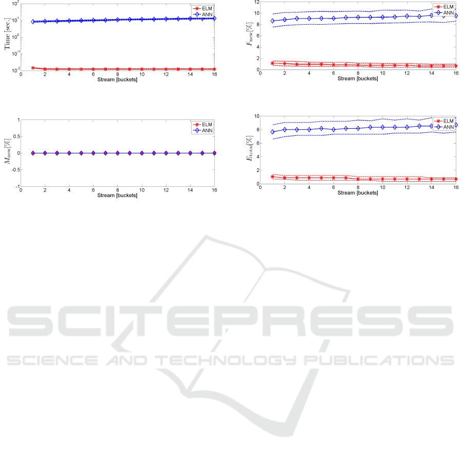
Figure 1: The time required for each bucket, i.e. classifica-
tion and retraining of both classifiers.
Figure 2: The rate of missed novelties for the incremental
ELM and the AANN, respectively.
F
n
is the number of novel class samples that the clas-
sifier fails to detect and falsely labels them as existing
classes. It corresponds to the number of false nega-
tives for one class classifiers. N
c
represents the num-
ber of samples which belong to the novel class within
the presented samples. F
p
is the number of existing
class samples which are wrongly indicated as outliers
by the classifier. It corresponds to the number of false
positives for one class classifiers. The total number of
samples presented to the classifier is denoted by N. F
e
is the number of existing class samples that are mis-
classified as other existing classes. As seen from (24),
it is not necessary that E
total
corresponds to the sum of
M
new
and F
new
(Masud et al., 2011).
7 RESULTS
The run time of the classifier matches the expectations
(Fig. 1). Since the proposed algorithm is incremental,
it requires less time to adapt. In any case the process-
ing time of the incremental ELM is of the order of
some milliseconds which helps to apply it to online
data streams.
Fig. 2 shows that the values M
new
of both algo-
rithms are zero, i.e. no outlier or novelty has been
missed. This is important since the outliers are sup-
posed to be near the boundary of the sample distri-
butions of all classes and thus accepting them would
significantly affect the performance of the classifiers
in the next iterations. Fig. 3 shows the value of
F
new
, which is initially below 2 % for the proposed
algorithm whereas it starts at more than 8 % for the
AANN. The rate of false detections by the incremen-
Figure 3: The rate of falsely detected novelties for the in-
cremental ELM and the AANN, respectively.
Figure 4: The total error rate for the incremental ELM and
the AANN, respectively.
tal ELM decreases with an increasing amount of train-
ing data, reaching a final level of less than 1 %. In
the case of the AANN, F
new
is increasing to more
than 9%. Although this means that a small fraction
of about 1–2 % of the samples belonging to known
classes is supposed to be outliers and, consequently,
they are rejected, this is not critical. In fact, this
removes the 1–2 % most extreme samples from the
semi-supervised training set and thus prevents possi-
bly false labels or sloppily performed gestures from
entering the training set. This leads to a slow gradual
adaptation of the learned sample distributions, lead-
ing to a final stabilised value reflected by E
total
(Fig.
4). This behaviour is favourable in slowly concept-
drifting data streams where the sample distributions
change slowly over time. The auto-encoder, in con-
trast, rejects more samples, which leads to a very slow
adaptation. The effect of this novelty detection step is
directly apparent in the total error E
total
of both clas-
sifiers. Initially, the error of the proposed approach
is around 1 % and decreases to less than 1 %. On
the other side, the total error of the auto-encoder is
initially around 8 % and increases with an increasing
F
new
.
8 SUMMARY AND CONCLUSION
We have presented an incremental neural network in
a semi-supervised learning scenario. In particular, we
have applied it to data streaming of emblematic arm
gestures, where it is possible that new classes appear
based on the continuously streamed data. This re-
laxes the need for a large and costly manually labelled
Neural Network based Novelty Detection for Incremental Semi-supervised Learning in Multi-class Gesture Recognition
295

data set. Using EVT, the algorithm uses a class-wise
statistical threshold for the rejection of outliers. It
thus does not require additional labelled data to de-
rive thresholds. More important, it works with mul-
tiple classes, and the normalisation prior to the EVT
ensures a class-wise threshold. Additionally, it is able
to separate the linearly unseparable gesture data. Im-
provements in the accuracy and processing time are
expected when applying this method to other types of
data. It might also be helpful for online fault detection
in industrial production processes.
REFERENCES
Al-Behadili, H., W
¨
ohler, C., and Grumpe, A. (2014).
Semi-supervised learning of emblematic gestures. At-
Automatisierungstechnik, 62(10):732–739.
Al-Behadili, H., W
¨
ohler, C., and Grumpe, A. (2015). Ex-
treme learning machine based novelty detection for
incremental semi-supervised learning. In 3’rd Inter-
national conference on image Information Processing
(ICIIP), page In Press. IEEE.
Clifton, D. A., Clifton, L. A., Bannister, P. R., and
Tarassenko, L. (2008). Automated novelty detec-
tion in industrial systems. In Advances of Computa-
tional Intelligence in Industrial Systems, pages 269–
296. Springer.
Fisher, R. A. and Tippett, L. H. C. (1928). Limiting forms
of the frequency distribution of the largest or smallest
member of a sample. In Mathematical Proceedings
of the Cambridge Philosophical Society, volume 24,
pages 180–190. Cambridge Univ Press.
Hertz, J., Krogh, A., and Palmer, R. G. (1991). Introduction
to the theory of neural computation, volume 1. Basic
Books.
Huang, G., Song, S., Gupta, J., and Wu, C. (2014).
Semi-supervised and unsupervised extreme learn-
ing machines. IEEE Transactions on Cybernetics,
44(12):2405–2417.
Huang, G.-B., Chen, L., and Siew, C.-K. (2006a). Universal
approximation using incremental constructive feed-
forward networks with random hidden nodes. IEEE
Transactions on Neural Networks, 17(4):879–892.
Huang, G.-B., Zhu, Q.-Y., and Siew, C.-K. (2006b). Ex-
treme learning machine: theory and applications.
Neurocomputing, 70(1):489–501.
Hugueny, S., Clifton, D. A., and Tarassenko, L. (2009).
Novelty detection with multivariate extreme value the-
ory, part ii: An analytical approach to unimodal esti-
mation. In Proc. MLSP, pages 1–6. IEEE.
Johnson, R. and Zhang, T. (2015). Semi-supervised learn-
ing with multi-view embedding: Theory and applica-
tion with convolutional neural networks. Proc. CoRR.
Kardaun, O. J. (2005). Classical methods of statistics: with
applications in fusion-oriented plasma physics, vol-
ume 1. Springer Science & Business Media.
Kendall, W. S., Marin, J.-M., and Robert, C. P. (2007). Con-
fidence bands for brownian motion and applications
to monte carlo simulation. Statistics and Computing,
17(1):1–10.
Lan, Y., Soh, Y. C., and Huang, G.-B. (2009). Ensemble of
online sequential extreme learning machine. Neuro-
computing, 72(13):3391–3395.
Li, K., Zhang, J., Xu, H., Luo, S., and Li, H. (2013). A semi-
supervised extreme learning machine method based
on co-training. Journal of Computational Information
Systems, 9(1):207–214.
Masud, M. M., Gao, J., Khan, L., Han, J., and Thuraising-
ham, B. (2011). Classification and novel class detec-
tion in concept-drifting data streams under time con-
straints. IEEE Transactions on Knowledge and Data
Engineering, 23(6):859–874.
Pimentel, M., Clifton, D., Clifton, L., and Tarassenko, L.
(2014). A review of novelty detection. Signal Pro-
cessing, 99:215–249.
Rao, C. R. and Mitra, S. K. (1971). Generalized inverse of
matrices and its applications, volume 7. Wiley New
York.
Richarz, J. and Fink, G. A. (2011). Visual recognition of
3d emblematic gestures in an hmm framework. Jour-
nal of Ambient Intelligence and Smart Environments,
3(3):193–211.
Roberts, S. J. (1999). Novelty detection using extreme value
statistics. IEE Proceedings-Vision, Image and Signal
Processing, 146(3):124–129.
Sakic, D. (2012). Semi-supervised learning using ensemble
methods gestures recognition. Master’s thesis, Uni-
versity of Dortmund.
Tax, D. (2001). One-class classification: concept-learning
in the absence of counter-examples. PhD thesis, TU
Delft, Delft University of Technology.
Tax, D. (2015). Ddtools, the data description toolbox for
matlab.
Tax, D. M. J. and Duin, R. P. W. (1999). Support vector do-
main description. Pattern Recognition Letters, 20(11-
13):1191–1199.
Yusoff, Y. A., Basori, A. H., and Mohamed, F. (2013). In-
teractive hand and arm gesture control for 2d med-
ical image and 3d volumetric medical visualization.
Procedia-Social and Behavioral Sciences, 97:723–
729.
Zhu, X. and Goldberg, A. B. (2009). Introduction to semi-
supervised learning. Synthesis lectures on artificial
intelligence and machine learning, 3(1):1–130.
VISAPP 2016 - International Conference on Computer Vision Theory and Applications
296
