Fluid Simulation by the Smoothed Particle Hydrodynamics Method: A

Survey

T. Weaver and Z. Xiao

Centre for Digital Entertainment, National Centre for Computer Animation, Bournemouth University, Bournemouth, U.K.

Keywords:

SPH, Computer Graphics, GPU, CUDA, CFD, Physically-based Simulation, Fluid Simulation.

Abstract:

This paper presents a survey of Smoothed Particle Hydrodynamics (SPH) and its use in computational ﬂuid

dynamics. As a truly mesh-free particle method based upon the Lagrangian formulation, SPH has been applied

to a variety of different areas in science, computer graphics and engineering. It has been established as a pop-

ular technique for ﬂuid based simulations, and has been extended to successfully simulate various phenomena

such as multi-phase ﬂows, rigid and elastic solids, and ﬂuid features such as air bubbles and foam. Various

aspects of the method will be discussed: Similarities, advantages and disadvantages in comparison to Eulerian

methods; Fundamentals of the SPH method; The use of SPH in ﬂuid simulation; The current trends in SPH.

The paper ends with some concluding remarks about the use of SPH in ﬂuid simulations, including some of

the more apparent problems, and a discussion on prospects for future work.

1 INTRODUCTION

Fluid simulation is utilised in many applications in-

cluding video games, special effects in both ﬁlm and

television, medical and military simulations, and vir-

tual reality. Some applications use a technique known

as ofﬂine rendering, where the scene or effect is ren-

dered by a large array of computers prior to its use

in the application. This can take a varying amount

of time depending on the complexity of the simula-

tion, and how many particles are used. The simula-

tion of ﬂuids in real-time is a challenging area, with

early examples using SPH reproducing relatively sim-

ple scenes such as calm bodies of water, gas inter-

action, and static smoke or fog. More recent imple-

mentations consider more of the properties that inﬂu-

ence ﬂuid behaviour such as splashing, bubbles, cor-

rect pressure representation, mixing of different ﬂuid

viscosities, and boiling and evaporation. As the avail-

able computing power has increased, achieving reli-

able frame rates in real-time simulations has become

possible. However, because the complexity of the

simulations has also increased there is still many areas

that could beneﬁt from research and reﬁnement.

The development of parallel computing, through

Application Programming Interfaces (APIs) such as

CUDA and OpenCL, has been widely accepted by

researchers for use in ﬂuid simulation. In general

terms, a simulation is made up of n particles, and for

each particle a set of equations must be solved each

frame before the simulation can be updated and ren-

dered. Solving the equations on the CPU means that

these calculations are solved linearly, one after an-

other, which for large values of n would heavily in-

crease the time taken to process each update. Utilis-

ing parallel computing means that for any number of

n particles, each particle equation could be solved in

parallel, reducing the time taken to perform all calcu-

lations. Furthermore, some of the more complex pro-

cesses used in ﬂuid simulation such as Nearest Neigh-

bour searching, and surface reconstruction/extraction

can be executed entirely on the GPU, discussed fur-

ther in Section 4.2.

Smoothed Particle Hydrodynamics is one of the

most popular methods in physically-based ﬂuid sim-

ulation. As the subject of this paper, SPH was cho-

sen for a number of reasons: realistic simulations in

real-time are achievable; a number of commercial 3D

graphical applications for simulating ﬂuid already use

SPH; and it is not only limited to ﬂuid based appli-

cations, some recent research using SPH include -

the calculation of protein-ligand binding rates in Bio-

Physics (Pan et al., 2015), modelling the sound of a

rigid body falling on water in Acoustics (Zhang et al.,

2015), and for the estimation of sea wave impact on

coastal structures in Coastal Engineering (Altomare

et al., 2015).

Weaver, T. and Xiao, Z.

Fluid Simulation by the Smoothed Particle Hydrodynamics Method: A Survey.

DOI: 10.5220/0005673702130223

In Proceedings of the 11th Joint Conference on Computer Vision, Imaging and Computer Graphics Theory and Applications (VISIGRAPP 2016) - Volume 1: GRAPP, pages 215-225

ISBN: 978-989-758-175-5

215

Figure 1: SPH simulation of a dam-break using 5000 particles executed entirely on the CPU averaging 40 fps.

2 SMOOTHED PARTICLE

HYDRODYNAMICS

Smoothed Particle Hydrodynamics, herein referred to

as SPH, was outlined in a series of papers by (Lucy,

1977) and (Gingold and Monaghan, 1977) to simulate

nonaxisymmetric phenomena in astrophysics. Using

SPH, the authors were able to calculate spatial deriva-

tives using analytical differentiation of interpolation

formulae. This offered a vast improvement over other

methods such as Particle in Cell, which utilises a grid

structure in order to calculate the spatial derivatives.

Additionally, speciﬁc particle attributes such as mo-

mentum, or pressure gradients, are found by sets of

differential equations with the latter being calculated

as the force between particle pairs.

Due to the extensibility and adaptability of SPH

it has been widely adopted to realistically simulate

a wide array of different ﬂuid simulations and ﬂuid

phenomena such as the experiment illustrated in Fig-

ure 1. The next section discusses some key factors

to consider when implementing SPH, including ker-

nel functions, smoothing radius, boundary conditions,

nearest neighbour searching, and time step evaluation.

2.1 SPH Fundamentals

As previously stated SPH is an interpolation method,

which uses a set of disordered points (the particles) to

express a function in terms of its values. The integral

interpolant of any function A(r) is deﬁned by

(r) =

Ω

A(r

)W(r − r

,h)dr

(1)

where the integration is over the entire space Ω, r is

any point in the space, and W is a smoothing kernel

with h width.

The integral interpolant can also be approximated

by a summation interpolant, given by

(r) =

∑

W(r − r

,h) (2)

where b denotes a particle, and the summation is over

all particles. Particle b has the following attributes:

mass m

, position r

, density ρ

, velocity v

, and the

value of any quantity A at r

is denoted by A

It is important to understand that this means a

differentiable interpolant of a function can be con-

structed from its values at the particles (interpolation

points), by using a kernel that is differentiable (Mon-

aghan, 1992). Thus any derivatives of this interpolant

can be obtained using standard differentiation, which

infers there is no need for grids or ﬁnite difference

methods.

Some “golden” rules to be considered in the SPH

method were presented in the early stages of research

(Monaghan, 1992): It is always best to assume the

kernel is Gaussian, and it is better to rewrite formulae

with the density placed inside of the operators. Al-

though the ﬁrst rule should be assumed as best prac-

tice, it would appear that while Gaussian kernels have

good mathematical properties they do not have a com-

pact support and require evaluations of exponential

functions which is further discussed in Section 2.2.

The second rule is used more frequently in modern

SPH, since it allows obtaining higher accuracy on the

gradient of a quantity ﬁeld (Kelager, 2006).

Calculating the pressure exerting on a particle is

an important part of the SPH process, as it may in-

ﬂuence how the particles react to one another, and

therefore how the simulation behaves. To calculate

the pressure at a particle the density must ﬁrst be cal-

culated, the pressure can then be determined using

the ideal gas state equation p = kρ, where k is a gas

stiffness constant that can be inﬂuenced by the num-

ber of particles in the ﬂuid or the temperature. How-

ever, with the consideration of the rest density of the

pressure, a modiﬁed equation had been rewritten to

p = k(ρ − ρ

) (M

uller et al., 2003). The revision to

the equation is much more suited to the simulation of

ﬂuid as the initial equation was formalised to model

gas, where particles emit a more repulsive reaction

to neighbours. In ﬂuid the particles would exhibit a

more cohesive reaction and also have a constant mass-

GRAPP 2016 - International Conference on Computer Graphics Theory and Applications

216

density at rest.

When the pressure at each particle is known, the

application of the SPH rule to the pressure term −∇p

at particle i is deﬁned by

= −∇p(r

) = −

∑

j6=i

∇W(r

− r

,h) (3)

However, this does not result in a symmetrical force,

which is apparent when two particles interact. This is

due to the particles only using one another to compute

their respective forces. Changing the form to

= −

∑

j6=i

+ p

2ρ

∇W(r

− r

,h) (4)

to compute the pressure is not only fast and stable, but

symmetry is guaranteed by using the arithmetic mean

of the pressure between interacting particles (M

uller

et al., 2003).

The calculation of viscosity is another important

factor to consider in SPH, each type of ﬂuid has its

own strength of viscosity, e.g. water vs oil, and this

must be modelled effectively. Viscosity is deﬁned as

the resistance to ﬂow, and in SPH the viscosity coefﬁ-

cient µ deﬁnes the strength of how viscous the liquid

is. In SPH terms the viscosity force term is deﬁned by

= µ∇

u(u

) = µ

∑

j6=i

∇

W(r

− r

,h) (5)

and much like the pressure force this is also an asym-

metric force due to the velocity ﬁeld variance between

particles. A Similar form has also been introduced for

force calculation, by including velocity differences as

deﬁned below (M

uller et al., 2003).

= µ

∑

j6=i

− v

∇

W(r

− r

,h) (6)

This achieves symmetry because the viscosity forces

only rely on the velocity differences, not the absolute

velocities. Viscosity is further discussed in Section

3.4.

Some of the equations necessary for implement-

ing SPH have been detailed in this section, a pseudo-

code overview of a basic SPH simulation loop step

provided by (Ihmsen et al., 2014) can be seen in Al-

gorithm 1. This algorithm uses a state equation, so

can be referred to as State-Equation SPH (SESPH).

2.2 Kernel Functions and Smoothing

Radius

There are many similarities between the use of

smoothing kernels in SPH, and difference schemes in

ﬁnite difference methods (Monaghan, 1992). The se-

lection of kernels for use within the SPH simulation is

Algorithm 1: SPH Simulation Loop.

1: for all particles i do

2: ﬁnd neighbours j

3: for all particles i do

4: ρ

∑

5: compute p

using ρ

6: for all particles i do

7: F

pressure

= −

∇p

8: F

viscosity

= m

ν∇

9: F

other

= m

10: F

(t) = F

pressure

+ F

viscosity

+ F

other

11: for all particles i do

12: v

(t + ∆t) = v

(t) + ∆tF

(t)/m

13: x

(t + ∆t) = x

(t) + ∆tv

(t + ∆t)

an important one since it may have a positive or nega-

tive effect on the accuracy produced, or the time taken

to perform the calculations and render the result. One

advantage using kernels in SPH is the kernel can be

calculated in a subroutine, meaning that interchang-

ing kernels to assess their suitability to the simulation

is trivial.

Monaghan suggested that a suitable kernel should

be normalised

W (r,h) = W (-r, h) (7)

and even

Ω

W (r, h)dr = 1 (8)

If both are satisﬁed then the interpolation is of sec-

ond order accuracy. Furthermore, it is suggested that

the kernel should have a limited or compact support

range, this ensures that the kernel does not interact

outside of the computational range of the deﬁned ra-

dius. It is suggested that the kernel should also be

positive to ensure that it is an averaging function, and

if the kernel is even then rotational symmetry is en-

forced (Sporring et al., 2005). Another suggestion is

that the kernel should also be monotonically decreas-

ing, and that it should satisfy the Dirac delta function

condition as h → 0 (Liu et al., 2003), as deﬁned be-

low:

lim

h→0

W(x − x

,h) = δ(x − x

) (9)

The smoothing radius h, and smoothing kernel W,

used in SPH are important considerations to ensure

a stable and robust simulation, and are subject to ad-

justment by changing the time or space. The problem

of ﬁnding a suitable smoothing radius is analogous to

deciding on the amount of particles that a SPH sim-

ulation should include. If h → ∞ then the simula-

tion can become unstable due to the kernel weighting

particle contributions less at the centre of the search

Fluid Simulation by the Smoothed Particle Hydrodynamics Method: A Survey

217

radius. Conversely, if h → 0 then not enough parti-

cles will be used in the weighting performed by the

kernel, and the results again will be imprecise. Al-

though some methods of ﬁnding a suitable value of h

exist, some experimentation may be required to ﬁnd

the optimum level at which the simulation behaves ac-

cordingly, while maintaining low computation times.

Considering h as a spherical radius, calculate the op-

timum size such that x particles comfortably ﬁll the

spherical volume, then choose a suitably small num-

ber of x such that the ﬂuid simulation is stable and

behaves accordingly, while still maintaining the prop-

erties of the chosen ﬂuid (Kelager, 2006).

2.3 Boundary Conditions

Fluid simulation implementing SPH should effec-

tively detect and respond to collisions between the

ﬂuid particles, known as ﬂuid-ﬂuid interaction, and

with the boundary (container) and any rigid objects

or meshes placed in the scene, known as ﬂuid-rigid

interaction. A simple method of collision response to

ﬂuid-rigid interaction is to reﬂect the colliding parti-

cle and its current velocity perpendicularly to the ob-

ject surface, generally calculated via the surface nor-

mal of the object at the point of contact. The simplic-

ity of this method is also its disadvantage, when the

boundary comprises of a simple ﬂat plane this method

can be reliable for small simulations. But when more

complex shapes are used or the simulation size is large

it can lead to discrepancies in calculations, where the

particles behave erratically or simply pass through the

object.

Furthermore, Having a perfectly elastic collision

is generally not advised, since ﬂuid does not behave

this way in nature, and as such the velocity should

be subject to division or multiplication by a restitu-

tion coefﬁcient. There are a variety of methods avail-

able to effectively manage particle interaction with

the boundary and other rigid objects in the simula-

tion space, since computing interaction via kernels

can cause some instability and clip parts of the ob-

ject entirely. Many of these methods generate static

particles, known as ghost or mirror particles, at the

surface of the object that have a repulsion force to re-

pel any incoming ﬂuid particles. In the next paragraph

some of the more recent contributions to the study of

boundary handling in SPH will be discussed.

One such method involves the addition of an in-

terface between the ﬂuid and the boundary, deﬁned

as a surface between the two adjacent materials, and

then deﬁne three boundary conditions (M

uller et al.,

2004):

1. No-Penetration Condition: No ﬂuid is allowed to

cross the boundary,

(

∂

∂t

u − v) · n = 0 at the boundary Γ (10)

2. No-Slip Condition: Models friction between the

ﬂuid and the solid,

(

∂

∂t

u − v) × n = 0 at the boundary Γ (11)

3. Actio = Reactio: The traction forces of the solid

must be opposite to that of the ﬂuid on the bound-

ary Γ,

= σ

n = σ

(−n) = −g

(12)

By incorporating density estimated at the boundary

into the pressure forces acting on the ﬂuid, while

maintaining the ability to predict and correct the par-

ticle positions. It is also possible to prevent par-

ticle stacking and smoother density distributions at

the boundaries (Ihmsen et al., 2010). By replacing

the boundary entirely with particles which interact

with the ﬂuid with a prescribed force, simulations

can easily replicate interaction between the ﬂuid mass

and any rigid bodies, that may also ﬂoat (Monaghan,

2005). By sampling the solid boundary simulating

air particles with “ghost particles”, this can correctly

simulate cohesion between the ﬂuid and solid ob-

jects while reducing the amount of artifacts produced

(Schechter and Bridson, 2010). A similar approach

uses “mirror-particles”, the domain is discretised us-

ing a set of triangles for ease of calculating the normal

directions, the mirror-particles are generated when a

particle is found to be within a certain threshold of the

triangle (Napoli et al., 2015).

Similarly, a coupled, dynamic solid boundary

treatment approach can be used where the boundaries

of the domain are padded with an inner layer of parti-

cles that exhibit a repulsive force, and two outer lay-

ers of ghost particles (Chen et al., 2015). Some of

these approaches can suffer with inhomogeneous par-

ticle sampling, but this can be solved by deriving new

equations which consider the boundary particles rela-

tive contribution to a physical quantity. This can also

improve the particle initialisation at complex bound-

aries and the boundary resampling of any dynamic ob-

jects in the simulation (Akinci et al., 2012).

2.4 Nearest Neighbour Searching

In order to effectively calculate forces between par-

ticles SPH necessitates using a Nearest Neighbour

search algorithm to locate any particles that may inﬂu-

ence the root particle. Illustrated in Figure 2, Nearest

Neighbour searching is an extremely computationally

expensive operation, and as such can have a largely

GRAPP 2016 - International Conference on Computer Graphics Theory and Applications

218

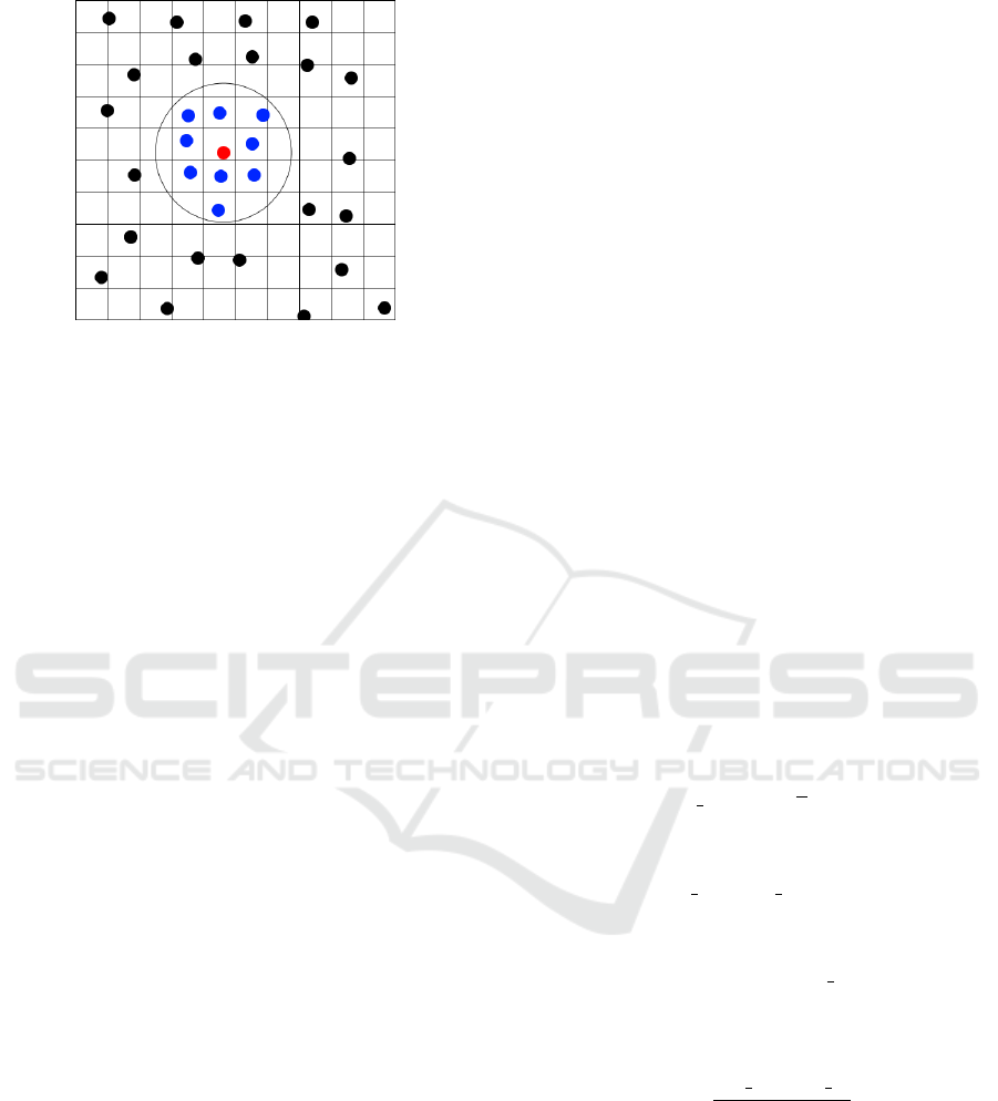
Figure 2: 2D grid-based nearest neighbours: the root par-

ticle shown in red and its neighbouring particles shown in

blue within a deﬁned search radius, the black particles out-

side would not be considered in pressure and viscosity cal-

culations.

negative impact on the time taken to process each

frame. It is advised to utilise a method of spatial de-

composition so that the entire set of particles need not

be iterated over to ﬁnd a speciﬁc instance. Spatial de-

composition offers a method of dividing the working

space of the simulation into smaller sections, gener-

ally referred to as voxels or cells, that can be accessed

directly using a divisor such as position in 3D space,

or lookup key.

A popular method of Nearest Neighbour searching

uses a 3D uniform grid, a bounding cube contains the

particles, and a twice division strategy to calculate the

optimum edge length of the grid cells. The expense

of performing sorting operations on the set can be re-

duced by using only certain query points, which in

turn reduces the necessary number of distance calcu-

lations required (Zhao et al., 2014) . Another popular

method is spatial hashing, the effectiveness is bound

by the speed with which the unique hash keys used

to represent each grid cell can be generated. But care

must be taken to ensure that there are no “hash colli-

sions”, where multiple hash keys map to the same grid

cell (Kelager, 2006). By using a sliced data structure

and the GPU to construct and access the stored val-

ues, the computational space is sliced into a number

of two-dimensional planes and an index, and a dy-

namic grid is constructed to ﬁt the particle distribution

with some margin (Harada et al., 2007).

Some methods can be executed entirely on the

GPU, using table lookup based Z-Indexing for range

queries and a virtual indexing grid for spatial subdi-

vision. The Z-Index is used to sort the particles and

any found within a power-of-two sized aligned block

are considered neighbours (Goswami et al., 2010). In

comparison with a number of techniques implement-

ing uniform grids that include index, parallel and Z-

Index sorting, and spatial and compact hashing. It

shows that Z-Indexing and compact hashing are both

equally efﬁcient methods, where the memory con-

sumption of the preceding scales with the domain, and

that of the proceeding with the number of particles

(Ihmsen et al., 2011) .

2.5 Numerical Time Integration & Time

Step

There are many different methods of numerical in-

tegration, and for clarity the most regularly imple-

mented will be brieﬂy discussed.

The Implicit Euler scheme is, contrary to its name,

a semi-implicit numerical integration method and is

based on the more commonly used explicit Euler

scheme. Unlike the explicit Euler, where the position

and velocity are updated in parallel, the positional up-

date utilises the result of the velocity calculation

t+∆t

= u

+ ∆ta

(13)

to estimate the new particle position

t+∆t

= r

+ ∆tu

(14)

The Leap-Frog scheme utilises the structure of the im-

plicit Euler method, and its name is derived from the

manner in which the velocities and positions “leap”

over one another. The initial velocity offset is calcu-

lated using a Euler step

−

∆t

= u

−

∆ta

(15)

with the regular velocity calculation given by

∆t

= u

t−

∆t

+ ∆ta

(16)

and the position calculated by

t+∆t

= r

+ ∆tu

∆t

(17)

In order to estimate a given velocity at arbitrary time

t a midpoint approximation can be used

≈

t−

∆t

+ u

∆t

(18)

Deciding on the most appropriate time step is an

important factor when considering time integrating

methods, since it can effect the stability of the inte-

gration. Due to the manner in which SPH utilises

regular differential equations, any stable method of

time stepping can be used. However, when there is

an absence of dissipation it would be beneﬁcial to

use a symplectic integrator such as the Verlet sec-

ond order integrator (Monaghan, 2005). Compar-

ing Weakly-Compressible SPH with Incompressible

Fluid Simulation by the Smoothed Particle Hydrodynamics Method: A Survey

219

SPH, the choice of time step is separate for each but

chosen by the same expression, to satisfy the min-

imum of three conditions: the Courant-Friedrichs-

Levy condition, and the mass and viscosity force

conditions (Lee et al., 2008). However, it is also

possible to control the time-step by using the afore-

mentioned CFL condition, gravity, viscosity and drag

terms (Monaghan, 2005).

2.6 Compressibility and SPH

The original formulation of the SPH method was de-

signed to model compressible ﬂow problems, but im-

plementing incompressibility is an important factor

when creating realistic simulations. Enforcing incom-

pressibility can be a computationally expensive step,

and can be achieved using a variety of different meth-

ods. One of the simpler methods solves an equation

of state using the density to derive the pressure. This

however has its disadvantages, one being that the time

step has to be extremely small, and another that non-

physical pressure ﬂuctuations caused by erroneous

density calculations can lead to numerical instability

in the simulation. Fully incompressible SPH aims to

rectify these issues by treating pressure and viscosity

forces separately. The pressure is calculated by pro-

jecting the intermediate velocity ﬁeld, found by inte-

grating the ﬁeld forward in time without enforcing in-

compressibility, onto a divergence-free space by solv-

ing a derived pressure Poisson equation (Cummins

and Rudman, 1999). Other methods include Weakly-

Compressible SPH (WCSPH), Implicit Incompress-

ible SPH (IISPH), Predictive-Corrective Incompress-

ible SPH (PCISPH), and Local-Poisson SPH (LC-

SPH).

By experimenting with a variety of simulations

including 2D lid-driven cavity ﬂow, ﬂow around a

bluff, and a series of dam-breaks, Incompressible

SPH out-performed the Weakly-Compressible, yield-

ing more reliable results with smoother velocity and

pressure ﬁelds (Lee et al., 2008). Further methods

have been applied to enhance the implementation of

Incompressible SPH, such as Moving Particle Semi-

Implicit methods and error compensating source of

the pressure Poisson equation (Gotoh et al., 2014).

Recently, a method named Predictive-Corrective

Incompressible SPH combining the advantages of

Weakly-Compressible SPH and Incompressible SPH,

low computational cost per update and a larger time

step has been presented (Solenthaler and Pajarola,

2009). It uses a prediction-correction scheme for

propagating estimated density values through the ﬂuid

until a user deﬁned density variation limit is reached,

and updates the particle pressures such that incom-

pressibility is enforced. Compared with WCSPH,

PCISPH achieves similar results with less computa-

tion, and also allows the use of much larger time steps

without sacriﬁcing the stability of the simulation. Re-

cent studies have shown that approaches combining

Implicit-Incompressible SPH with another popular

method of ﬂuid simulation known as Fluid-Implicit-

Particle (FLIP), have several advantages compared

with regular SPH including low memory usage, com-

putation time and larger time steps. The combination

of the two methods counteract the disadvantages of ei-

ther individually, with low memory consumption for

large scale simulations, and low computational com-

plexity (Cornelis et al., 2014).

To avoid the computational cost of solving a Pois-

son pressure equation globally, a Local Poisson SPH

method that retains the large time step of Incompress-

ible SPH has been introduced. It effectively elimi-

nates the large density deviations arising from solid

boundary treatment (He et al., 2012)

3 EXPERIMENTAL

APPLICATIONS

Recent research on SPH is primarily concerned with

reﬁning, or detailing new advances which improve the

algorithms used in creating the various simulations.

Although some research focuses on speciﬁc scenar-

ios where SPH is used such as viscous ﬂuids, multi-

phase ﬂuids, erosion modelling, and interactive ﬂuids.

Some of the recent research and developments will be

discussed in the proceeding subsections.

3.1 Multiphase Flows

Many SPH simulations are based upon “single-phase”

ﬂows, which is a single liquid interacting with bound-

aries or obstacles placed in the scene. Fluids with

more than one phase are called multiphase, and can

be classiﬁed as miscible, where the phases can freely

mix with one another; or immiscible where the phases

are separate, and cannot initiate a chemical reaction

between them. An example of miscible ﬂow would

be the mixing of two liquids with different viscosities

e.g. combining oil and vinegar, and immiscible ﬂow

e.g. lava ﬂows, water at boiling point. The separat-

ing axis in multiphase ﬂows is often referred to as an

interface of zero thickness that balances the separa-

tion of two phases using surface tension (Chen et al.,

2015).

After simulation of lava ﬂows and the dusty gas

produced in volcanic eruptions, it was noted that SPH

is particularly suitable for modelling multiphase ﬂow

GRAPP 2016 - International Conference on Computer Graphics Theory and Applications

220

due to the ease of modiﬁcation to handle gas, solid or

liquid phases, achieved with the inclusion of an en-

ergy equation (Monaghan and Kocharyan, 1995). By

further modifying the particle approximation step, in-

troducing a density re-initialisation treatment to cor-

rect any mass discontinuities occurring at the inter-

faces can also improve multi-phase ﬂow SPH. Parti-

cles residing close to the interfaces between phases

are treated as ghost particles for any particles from

neighbouring phases (Chen et al., 2015). In their

research, reﬁnement of the mixture model also im-

proves multi-phase simulation where the reliance on

tracking interfaces between the phases is replaced by

representing the phases with their volume fractions

(Ren et al., 2014). Each phase has its own set of par-

ticles that carry the mixture mass, velocity, and any

physical qualities of the phase to discretise the multi-

phase system.

3.2 Bubbles, Foam and Splashing

In ﬂuid simulation the representation of the ﬂuid is

of foremost importance. The addition of features that

ﬂuid creates in its movement such as bubbles, waves,

foam, water splashing and turbulence is also impor-

tant in creating realistic visualisations. Some may be

created when the ﬂuid interacts with solid objects in

its environment, or when something is introduced to

the ﬂuid e.g. a whisk or large object falling into the

ﬂuid. The computation required to represent these

features can be quite complex depending on the sim-

ulation, but the visualisation thereof is also a complex

task and can require a variety of different techniques

to render accurately.

In general, bubbles are created when air particles

get trapped within the ﬂuid, in the case of water which

has a low viscosity these bubbles would quickly rise

to the surface of the liquid possibly becoming foam.

In a more viscous liquid the bubbles may stay in place

creating an air pocket. This is due to a difference in

density, or rest-density, between the particles. When

two particle bodies of different density are mixed the

difference will cause the less dense ﬂuid to rise. Bub-

bles are able to be simulated using SPH by generating

air particles where air pockets are likely to form in the

ﬂuid, this can be extended to simulate boiling water

through phase transitions by tracking the temperature

and changing the type and density of the particles dy-

namically (M

uller et al., 2005). Multi-phase SPH for-

mulations are well suited to simulating bubbles and

foam, using a saturated function for volume allows

smaller and larger bubbles to behave differently, and

the inclusion of a drag force can effectively simulate

the two-way interaction between the phases. When

air particles reach the surface of the ﬂuid body they

are treated as foam particles that have a ﬁnite lifes-

pan before being removed. Detecting particles that

have breached the surface can be achieved using a

smoothed colour ﬁeld, or comparing the number of

neighbours using a deﬁned threshold (Akinci et al.,

2011).

Splashing or sloshing occurs when ﬂuid particles

leave the main body of ﬂuid, this can be the result of

ﬂuid interaction with solid boundaries or objects, and

user interaction with the ﬂuid. SPH is able to simulate

some instances of splashing in its original form, how-

ever this can be improved to simulate a much more

realistic representation, such as the introduction of

an error compensating source of the Poisson pressure

equation, and a higher order laplacian (Gotoh et al.,

2014). Apart from the robustness and stability that

SPH can offer for most of the simulations, to simulate

sparsely sampled thin features in free surface ﬂows

e.g. splashing, SPH might encounter difﬁculty to-

wards failure. By applying the combination of a free

surface energy function based surface tension force

schemes, efﬁcient air pressure calculation, and geom-

etry aware anisotropic kernels used to ﬁlter internal

pressure estimated at two scales, the simulation has

been enhanced and improved (He et al., 2014).

3.3 Interactive Fluids

Fluid interaction can take place between ﬂuid parti-

cles and a wide number of different mediums includ-

ing deformable solids or bodies, free surfaces, and

particles representing different ﬂuids or gases. SPH is

able to be combined with a Finite Element approach

to model the interactivity of ﬂuid particles and de-

formable solids, where boundary particles are placed

at the object surface according to Gaussian quadrature

rules (M

uller et al., 2004).

Particle-air interaction with SPH can be effec-

tively modelled by the calculation of the surface-

tension and adhesion forces, which removes the ne-

cessity of surface tracking and the use of ghost or vir-

tual particles (Akinci et al., 2013b). Another method

applies the generation of air particles where air pock-

ets are likely to be formed in the liquid. The inclusion

of temperature calculations to adjust particle types

and densities means phenomena such as boiling water

can also be modelled (M

uller et al., 2005).

Fluid interaction with soluble objects where the

object is composed entirely of particles, can be mod-

elled with SPH via the inclusion of a dissolution

model. During dissolution the object particle con-

centration is transferred to the adjacent ﬂuid parti-

cles until the object particle is completely dissolved,

Fluid Simulation by the Smoothed Particle Hydrodynamics Method: A Survey

221

at which point it detaches from the object (Kim and

Park, 2014).

3.4 Viscous, Elastic Fluids and Objects

Viscous, and Viscoelastic ﬂuids in SPH include sub-

stances such as oil, honey, blood, and lava. Flu-

ids can be subject to dynamic alteration due to tem-

perature changes including melting, freezing into a

solid, and viscosity ﬂuctuations in ﬂow which will

change the behaviour and appearance of the ﬂuid.

Although SPH can model viscous ﬂuids, a problem

known as tensile instability can arise due to the cohe-

sive pressure which can cause the particles to cluster

or become sparsely distributed. The tensile instabil-

ity problem is able to be rectiﬁed with the use of a

hyperbolic-shaped kernel that possesses non-negative

second derivatives, which ensures even distribution of

particles in the ﬂuid (Yang et al., 2014).

The simulation of bubbles and air particles in

particularly viscous liquids can be problematic, but

through the use of multi-phase SPH formulations it

is possible to compute the two-phase ﬂow inside and

outside of the bubble which addresses the large den-

sity differences, and surface tension is able to be en-

forced using a Continuum Surface Force. Improving

the efﬁciency and robustness of viscous ﬂuid simu-

lations using SPH has been achieved via the implicit

integration of viscosity, and the conversion to a sparse

linear system with a symmetric positive matrix (Taka-

hashi et al., 2015). Other improvements include the

reconstruction of the velocity ﬁeld from the target ve-

locity gradient, where any density corrections from

the preceding pressure projection stage are preserved

meaning only one pressure projection step is required

(Peer et al., 2015). Both revisions improve the simu-

lation reliability, and results, with the phenomena of

buckling and coiling and multi-phase viscous liquid

mixing correctly represented.

Elastic-solid coupling using SPH ﬂuids can be

achieved by sampling the triangulated surfaces of

solids using boundary particles, but can suffer from

problems when using deformable boundaries such as

spatial and temporal discontinuities and particle leak-

ing through boundaries. A method of countering this

is through the use of speciﬁc surface tension and ad-

hesion forces which do not rely on the introduction of

ghost particles (Akinci et al., 2013b).

Using SPH to model objects or solids in simula-

tions is also popular, ﬁnding use in deformable ob-

jects and meshes, and elastic and plastic objects. As

the object can be represented entirely by the parti-

cles, processes such as handling large deformations,

adding special conditions such as repulsion forces, or

simulating the ﬂuid body interacting with the solid is

relatively simple. A method often used in Finite El-

ement Methods, the corotational formula, has been

adapted for use in modelling meshless deformable

solids with SPH. The rotations in the deformation

ﬁeld are computed using a variant of the shape match-

ing approach adapted for use with SPH (Becker et al.,

2009). Compared with similar methods, the corota-

tional approach not only improves the realistic be-

haviour of the simulation, but also the range of elasto-

mechanical properties that can be simulated.

4 CURRENT TRENDS IN SPH

Since its creation, SPH has been adapted and modi-

ﬁed to suit a variety of research areas. With exten-

sions to the original model it has proved extremely

adaptive, ﬁnding use in various areas including sound

and acoustics research, naval engineering and bio-

engineering. This section aims to look at a selected

number of areas currently popular with researchers in

ﬂuid dynamics.

4.1 Surface Reconstruction

Surface reconstruction is an important research topic

in SPH. The body of the ﬂuid is represented by the

particles in the simulation, but to render these as a

body of ﬂuid the particle surfaces must be extracted.

This is a computationally expensive operation when

constructing a high resolution, detailed and artifact

free surface from large sets of particles and is often

seen as a bottleneck due to the complexity and high

memory usage.

Some of the most widely adopted methods involve

algorithms such as marching cubes or tiles, and ray-

tracing. The main problem with marching cubes is the

high memory usage and wastage, which can impact

execution times and results. The Histogram Pyramid

Marching Cubes algorithm removes any cells which

contain no triangles which improves on the mem-

ory consumption, and can also be implemented on

the GPU, greatly improving execution times (Huang

et al., 2015).

There are also methods that reconstruct the sur-

faces from grids and anisotropic kernels. With each

particle represented by anisotropic kernels, marching

cubes is used to construct a mesh that approximates

the ﬂuid surface, with additional diffusion smoothing

steps to account for any bumpiness on the surface (Yu

and Turk, 2010).

Three-level grids have been used for surface re-

construction on the CPU (Akinci et al., 2013a) and

GRAPP 2016 - International Conference on Computer Graphics Theory and Applications

222

more recently on the GPU, where the execution time

was vastly improved due to parallelisation. Using a

grid can lead to cracks in the approximated surface

which appear in the common faces between adjacent

grid cells, so techniques must account for this with

some approaches dealing with it procedurally, de-

tecting and ﬁlling cracks at runtime (Du and Kanai,

2014). Surface reconstruction using Volume render-

ing makes further use of grids, resampling the particle

quantities onto a view volume sized 3D grid which is

stored as a 3D texture which can be stored and used

on the GPU for ray casting (Fraedrich et al., 2010).

4.2 GPU Utilisation

The computational complexity of ﬂuid simulation is a

challenging area and one that prevents truly real-time

simulations from achieving good graphical ﬁdelity.

To correctly model ﬂuid the simulation should com-

prise of a relatively large number of particles and the

complexity scales with this. SPH is less dependent on

data and well suited for parallelisation, as are methods

it relies on such as Nearest Neighbour searching and

Surface Extraction/Reconstruction. Parallel process-

ing can be achieved using multi-core CPUs and mul-

tithreading, ﬁeld programmable gate arrays (FPGA),

Gravity Pipes (GRAPE) and the GPU. Multicore

CPUs and powerful GPUs are now commonplace in

most personal computers available and as such are

the most accessible forms of parallel computing, with

the GPU exhibiting the best price-performance ra-

tio. The parallelisation of SPH has seen an increas-

ing amount of research as the programmability of the

GPU has become more accessible using languages

such as NVIDIA’s CUDA and OpenCL.

Approaches executing the entire simulation on the

GPU can be achieved by removing the data depen-

dencies and changing the computational model from

“gathering” to “distributing”. Adaptive sampling is

used to allow focusing of computation on speciﬁc ar-

eas in the ﬂuid, and particle merging to reduce the

overall number of particles (Zhang et al., 2008). GPU

implementations can also beneﬁt from optimisations

regarding how positional and neighbourhood data is

stored on the GPU (Rustico et al., 2014), and ensuring

data representation is optimised for use by the GPU.

For instance, particle data can maintain contiguity if

an Array of Structures (AoS) format is used. But as

not all particle attributes are accessed simultaneously

a Structure of Arrays (SoA) format achieves a higher

memory bandwidth on the GPU (Nie et al., 2015).

To extend the previous work executed on single

GPU systems (H

erault et al., 2010), an optimisation

method was utilised in considering updating how po-

sitional and neighbourhood data is stored to better suit

GPU memory access, and the replacement of depre-

cated functions no longer supported in CUDA (Rus-

tico et al., 2014). The proposed revision with a single

GPU implementation is more than twice as fast as the

original.

5 CONCLUSIONS

Smoothed Particle Hydrodynamics is a fully mesh-

free particle based method, where the particles carry

the material properties of the medium it is simulat-

ing (ﬂuid, gases). This paper has presented a survey

of the current state of SPH research and techniques,

some of the history of the SPH method, its applica-

tion in various ﬁelds, and some of the more recent

improvements.

The largest issue still facing researchers of SPH

is the computational overhead. Many of the sim-

ulations presented in papers involving a very large

number of particles or complex procedures are pre-

rendered. Advances made in computer hardware are

having a positive effect on this issue, and are en-

abling researchers to devise new strategies and tech-

niques to improve the execution times, but it will

likely not completely resolve this issue. Furthermore,

reﬁnement of the algorithms used and development of

new algorithms will likely assist in the contribution

of reducing the complexity. Simulations executed on

the GPU is an area that shows a lot of promise, as

SPH is well suited to parallel execution this offers a

large speed advantage over traditional execution on

the CPU.

As SPH is a purely particle based method, to sim-

ulate actual ﬂuid the particles need to be rendered

as such. Surface reconstruction is a technique for

achieving visualisation of ﬂuids and its complexity

scales with the number of particles used in the sim-

ulation. Furthermore, other time consuming calcula-

tions such as lighting and shadow effects, or surface

reﬂections used to create an aesthetically pleasing liq-

uid are an important consideration. Real-time sim-

ulations executed on the GPU using around 30,000

particles can maintain a steady average frame rate of

around 50 frames per second (fps), adding surface ex-

traction and rendering can reduce this by between 60-

80%. So, efﬁcient rendering could be considered a

bottleneck in ﬂuid simulation using SPH and would

beneﬁt from further research.

Fluid Simulation by the Smoothed Particle Hydrodynamics Method: A Survey

223

REFERENCES

Akinci, G., Akinci, N., Oswald, E., and Teschner, M.

(2013a). Adaptive surface reconstruction for sph us-

ing 3-level uniform grids.

Akinci, M., Julian, I., Gizem, B., and Teschner, M. (2011).

Animation of air bubbles with sph.

Akinci, N., Akinci, G., and Teschner, M. (2013b). Versa-

tile surface tension and adhesion for sph ﬂuids. ACM

Transactions on Graphics, 32.6:182.

Akinci, N., Ihmsen, M., Akinci, G., Solenthaler, B., and

Teschner, M. (2012). Versatile rigid-ﬂuid coupling for

incompressible sph. ACM Transactions on Graphics

(TOG), 31(4):62.

Altomare, C., Crespo, A. J., Domnguez, J. M., Gmez-

Gesteira, M., Suzuki, T., and Verwaest, T. (2015).

Applicability of smoothed particle hydrodynamics for

estimation of sea wave impact on coastal structures.

Coastal Engineering, 96:1–12.

Becker, M., Ihmsen, M., and Teschner, M. (2009). Coro-

tated sph for deformable solids. NPH, pages 27–34.

Chen, Z., Zong, Z., Liu, M. B., Zou, L., Li, H. T., and

Shu, C. (2015). An sph model for multiphase ﬂows

with complex interfaces and large density differences.

Journal of Computational Physics, pages 169–188.

Cornelis, J., Ihmsen, M., Peer, A., and Teschner, M. (2014).

Iisph-ﬂip for incompressible ﬂuids. Computer Graph-

ics Forum, 33(2).

Cummins, S. J. and Rudman, M. (1999). An sph projection

method.

Du, S. and Kanai, T. (2014). Gpu-based adaptive surface

reconstruction for real-time sph ﬂuids.

Fraedrich, R., Auer, S., and Westermann, R. (2010). Efﬁ-

cient high-quality volume rendering of sph data. Visu-

alization and Computer Graphics, 16.6:1533–1540.

Gingold, R. A. and Monaghan, J. J. (1977). Smoothed par-

ticle hydrodynamics: theory and application to non-

spherical stars. Monthly notices of the royal astro-

nomical society, 181.3s:375–389.

Goswami, P., Schlegel, P., Solenthaler, B., and Pajarola,

R. (2010). nteractive sph simulation and rendering

on the gpu. Proceedings of the 2010 ACM SIG-

GRAPH/Eurographics Symposium on Computer An-

imation.

Gotoh, H., Khayyer, A., Ikari, H., Arikawa, T., and Shi-

mosako, K. (2014). On enhancement of incompress-

ible sph method for simulation of violent sloshing

ﬂows. Applied Ocean Research, 46:104–115.

Harada, T., Koshizuka, S., and Kawaguchi, Y. (2007).

Sliced data structure for particle-based simulations on

gpus. Proceedings of the 5th international conference

on Computer graphics and interactive techniques in

Australia and Southeast Asia.

He, X., Liu, N., Li, S., Wang, H., and Wang, G. (2012).

Local poisson sph for viscous incompressible ﬂuids.

Computer Graphics Forum, 31(6):1948–1958.

He, X., Wang, H., Zhang, F., Wang, H., Wang, G., and

Zhou, K. (2014). Robust simulation of sparsely sam-

pled thin features in sph-based free surface ﬂows.

ACM Transactions on Graphics (TOG), 34.

erault, A., Bilotta, G., and Dalrymple, R. A. (2010). Sph

on gpu with cuda. Journal of Hydraulic Research,

48.S1:74–79.

Huang, C., Zhu, J., Sun, H., and Wu, E. (2015). Parallel-

optimizing sph ﬂuid simulation for realistic vr envi-

ronments. Computer Animation and Virtual Worlds,

26(1):43–54.

Ihmsen, M., Akinci, N., Becker, M., and Teschner, M.

(2011). A parallel sph implementation on multi-core

cpus. Computer Graphics Forum, 30:99–112.

Ihmsen, M., Akinci, N., Gissler, M., and Teschner, M.

(2010). Boundary handling and adaptive time-

stepping for pcisph. Workshop on virtual reality in-

teraction and physical simulation VRIPHYS.

Ihmsen, M., Orthmann, J., Solenthaler, B., Kolb, A., and

Teschner, M. (2014). Sph ﬂuids in computer graphics.

Eurographics - State of the Art Reports.

Kelager, M. (2006). Lagrangian ﬂuid dynamics using

smoothed particle hydrodynamics. University of

Copenhagen. Denmark.

Kim, S. and Park, J. (2014). A sph-based dissolution behav-

ior model for real-time ﬂuid-solid interaction. SIG-

GRAPH Asia 2014 Posters.

Lee, E.-S., Moulinec, C., Xu, R., Violeau, D., Laurence, D.,

and Stansby, P. (2008). Comparisons of weakly com-

pressible and truly incompressible algorithms for the

sph mesh free particle method. Journal of computa-

tional physics, 227:8417–8436.

Liu, M. B., Liu, G. R., and Lam, K. Y. (2003). Constructing

smoothing functions in smoothed particle hydrody-

namics with applications. Journal of Computational

and applied Mathematics, 155.2:263–284.

Lucy, L. B. (1977). A numerical approach to the test-

ing of the ﬁssion hypothesis. Astronomical Journal,

82:1013–1024.

Monaghan, J, J. and Kocharyan, A. (1995). Sph simulation

of multi-phase ﬂow. Computer Physics Communica-

tions, 87:225–235.

Monaghan, J. J. (1992). Smoothed particle hydrodynam-

ics. Annual review of astronomy and astrophysics,

30:543–574.

Monaghan, J. J. (2005). Smoothed particle hydrodynamics.

Reports on progress in physics, 68.8:1703–1759.

uller, M., Charypar, D., and Gross, M. (2003).

Particle-based ﬂuid simulation for interactive ap-

plications. Proceedings of the 2003 ACM SIG-

GRAPH/Eurographics symposium on Computer ani-

mation.

uller, M., Schirm, S., Teschner, M., Heielberger, B.,

and Gross, M. (2004). Interaction of ﬂuids with de-

formable solids. Computer Animation and Virtual

Worlds 15, no 3-4:159–171.

uller, M., Solenthaler, B., Keiser, R., and Gross, M.

(2005). Particle-based ﬂuid-ﬂuid interaction. Pro-

ceedings of the 2005 ACM SIGGRAPH/Eurographics

symposium on Computer animation, pages 237–244.

Napoli, E., Marchis, M. D., and Vitanza, E. (2015).

Panormus-sph. a new smoothed particle hydrodynam-

ics solver for incompressible ﬂows. Computers and

Fluids, 106:185–195.

GRAPP 2016 - International Conference on Computer Graphics Theory and Applications

224

Nie, X., Chen, L., and Xiang, T. (2015). Real-time incom-

pressible ﬂuid simulation on the gpu. International

Journal of Computer Games Technology.

Pan, W., Daily, M., and Baker, N. A. (2015). Numerical

calculation of protein-ligand binding rates through so-

lution of the smoluchowski equation using smoothed

particle hydrodynamics. BMC biophysics, 8.1.

Peer, A., Ihmsen, M., Cornelis, J., and Teschner, M. (2015).

An implicit viscosity formulation for sph ﬂuids. ACM

Transactions on Graphics, 34(4):114.

Ren, B., Li, C., Yan, X., Lin, M. C., Bonet, J., and Hu, S. M.

(2014). Multiple-ﬂuid sph simulation using a mixture

model. ACM Transactions on Graphics, 33 no. 5:171.

Rustico, E., Bilotta, G., Herault, A., Del Negro, C., and

Gallo, G. (2014). Advances in multi-gpu smoothed

particle hydrodynamics simulations. Parallel and Dis-

tributed Systems, IEEE Transactions, 25(1):43–52.

Schechter, H. and Bridson, R. (2010). Ghost sph for ani-

mating water. ACM Transactions on Graphics (TOG),

31(4):61.

Solenthaler, B. and Pajarola, R. (2009). Predictive-

corrective incompressible sph. ACM Transactions on

Graphics (TOG), 28(3).

Sporring, J., Henriksen, K., and Dohlmann, H. (2005).

Physics-based animation. Hingham: Charles River

Media.

Takahashi, T., Dobashi, Y., Fujishiro, I., and Nishita, T., a.

L. M. (2015). Implicit formulation for sphbased vis-

cous ﬂuids. Computer Graphics Forum, 34(2):493–

502.

Yang, X., Liu, M., and Peng, S. (2014). Smoothed particle

hydrodynamics modeling of viscous liquid drop with-

out tensile instability. Computers and Fluids, 92:199–

208.

Yu, J. and Turk, G. (2010). Reconstructing surfaces of

particle-based ﬂuids using anisotropic kernels. ACM

Transactions on Graphics, 32.1:5.

Zhang, Y., Solenthaler, B., and Pajarola, R. (2008). Adap-

tive sampling and rendering of ﬂuids on the gpu. Pro-

ceedings of the Fifth Eurographics/IEEE VGTC con-

ference on Point-Based Graphicsg.

Zhang, Y., Zhang, T., Li, T., and Wang, P. (2015). Smoothed

particle hydrodynamics approach for modeling sound

of a rigid body falling on water. The Journal of the

Acoustical Society of America, 137(4):2403.

Zhao, J., Long, C., Xiong, S., Liu, C., and Yuan, Z. (2014).

A new k nearest neighbours algorithm using cell grids

for 3d scattered point cloud. Elektronika ir Elek-

trotechnika, 20(1):81–87.

Fluid Simulation by the Smoothed Particle Hydrodynamics Method: A Survey

225