
Joint Color and Depth Segmentation based on Region Merging and
Surface Fitting
Giampaolo Pagnutti and Pietro Zanuttigh
Department of Information Engineering, University of Padova, Via Gradenigo 6B, Padova, Italy
Keywords:
Segmentation, Depth, Color, Kinect, NURBS.
Abstract:
The recent introduction of consumer depth cameras has opened the way to novel segmentation approaches
exploiting depth data together with the color information. This paper proposes a region merging segmentation
scheme that jointly exploits the two clues. Firstly a set of multi-dimensional vectors is built considering the 3D
spatial position, the surface orientation and the color data associated to each scene sample. Normalized cuts
spectral clustering is applied to the obtained vectors in order to over-segment the scene into a large number
of small segments. Then an iterative merging procedure is used to recombine the segments into the regions
corresponding to the various objects and surfaces. The proposed algorithm tries to combine close compatible
segments and uses a NURBS surface fitting scheme on the considered segments in order to understand if
the regions candidate for the merging correspond to a single surface. The comparison with state-of-the-art
methods shows how the proposed method provides an accurate and reliable scene segmentation.
1 INTRODUCTION
The growing diffusion of consumer depth cameras has
made depth acquisition available to the mass market
and has opened the way to the usage of depth data
in order to aid many image processing tasks. Among
them segmentation from visual data has always been
a challenging issue despite a huge amount of research
devoted to this problem. The 3D representation of the
acquired scene contained in depth data is very use-
ful for this task and recently various approaches for
the combined segmentation of depth and color data
have been proposed. This idea resembles how the hu-
man visual system works, in fact our brain combines
the disparity information between the views from two
eyes with color information and prior knowledge on
the recognized objects to get the scene structure.
Among the various segmentation techniques, one
of the best performing family of approaches is the
one based on normalised cuts spectral clustering (Shi
and Malik, 2000). It can be easily extended to the
joint segmentation of image and depth data by feed-
ing to the clustering scheme multi-dimensional vec-
tors containing both color and geometrical clues for
each sample (Dal Mutto et al., 2012a). In this way
a relatively reliable segmentation can be obtained but
it is often difficult to avoid an over-segmentation of
the scene and at the same time distinguish the var-
ious objects and surfaces in the scene. The pro-
posed approach starts from an over-segmentation per-
formed with spectral clustering and then applies a re-
gion merging scheme in order to obtain the final seg-
mentation. The idea is to consider each couple of
close segments and analyze the common contour. If
the contour regions are compatible the algorithm then
evaluates if the two segments are part of the same sur-
face. The evaluation is performed by fitting a Non-
Uniform Rational B-Spline (NURBS) model on the
union of the two segments and comparing the accu-
racy of the fitting with the one obtained on each of the
two merged regions alone. If the accuracy remains
similar the segments are probably part of the same
surface and the merging is accepted, otherwise it is
discarded. This NURBS fitting scheme correctly han-
dles surfaces with a complex shape, differently from
many approaches that assume the surfaces to be pla-
nar. The procedure is repeated in a tree structure until
no more merging operations are possible.
2 RELATED WORKS
The idea of using also the information from an asso-
ciated depth representation to improve segmentation
algorithm performances has been exploited in vari-
ous recent scene segmentation schemes, a review of
Pagnutti, G. and Zanuttigh, P.
Joint Color and Depth Segmentation based on Region Merging and Surface Fitting.
DOI: 10.5220/0005672700930100
In Proceedings of the 11th Joint Conference on Computer Vision, Imaging and Computer Graphics Theory and Applications (VISIGRAPP 2016) - Volume 4: VISAPP, pages 93-100
ISBN: 978-989-758-175-5
Copyright
c
2016 by SCITEPRESS – Science and Technology Publications, Lda. All r ights reserved
93
this family of approaches is contained in (Dal Mutto
et al., 2012b). Clustering techniques can easily be ex-
tended to joint depth and color segmentation by mod-
ifying the feature vectors as in (Bleiweiss and Wer-
man, 2009; Wallenberg et al., 2011; Dal Mutto et al.,
2011). In particular a segmentation scheme based on
spectral clustering that is able to automatically bal-
ance the relevance of color and depth clues has been
proposed in (Dal Mutto et al., 2012a).
Region splitting and growing approaches have
also been considered. In (Erdogan et al., 2012) su-
perpixels produced by an over-segmentation of the
scene are combined together in regions correspond-
ing to the planar surfaces using an approach based
on Rao-Blackwellized Monte Carlo Markov Chain.
The approach has been extended to the segmentation
of multiple depth maps in (Srinivasan and Dellaert,
2014). The top down approach (region splitting) has
been used in (Pagnutti and Zanuttigh, 2014) where
the segmentation is progressively refined in an itera-
tive scheme by recursively splitting the segments that
do not represent a single surface in the 3D space. Hi-
erarchical segmentation based on the output of con-
tour extraction has been used in (Gupta et al., 2014),
that also deals with object detection from the seg-
mented data. Another combined approach for seg-
mentation and object recognition has been presented
in (Silberman et al., 2012), that exploits an initial
over-segmentation with the watershed algorithm fol-
lowed by a hierarchical scheme.
A joint clustering method on the color, 3D po-
sition and normal information followed by a statis-
tical planar region merging scheme has been pre-
sented in (Hasnat et al., 2014). In (Ren et al., 2012)
a MRF superpixel segmentation is combined with a
tree-structured segmentation for scene labeling. Fi-
nally dynamic programming has been used in (Taylor
and Cowley, 2013) to extract the planar surfaces in
indoor scenes.
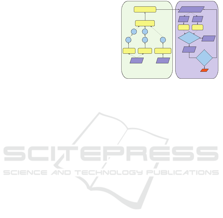
3 GENERAL OVERVIEW
Fig. 1 shows a general overview of the proposed ap-
proach. The color image and the depth map are firstly
converted to a unified representation consisting in a
set of 9D vectors containing the 3D position, the ori-
entation information and the color coordinates in the
CIELab color space of each sample. This represen-
tation is then over-segmented using both color and
depth information inside a framework based on spec-
tral clustering. The over-segmentation is fed into the
iterative region merging procedure. In this step firstly
a NURBS model is fitted over each segmented region.
! "#
!
$%
$%
$
&
'
&
(
(
)
*
*
+,
-
(
$%
+..
!
/
0*
.
-/
Figure 1: Overview of the proposed approach.
The algorithm then looks at all the adjacent regions,
checks if they can be considered for merging by look-
ing at the compatibility of the color and geometry val-
ues on the common contour. In this case it fits a para-
metric NURBS surface on the merged region. The
surface fitting error is computed and compared with
the weighted average of the fitting error on the two
merged pieces. If the error remains similar (i.e., the
two regions are part of the same surface) the merging
is accepted, if it increases (i.e., they probably belong
to two different surfaces), the merge is discarded. The
procedure is repeated iteratively in a tree structure un-
til no more merging operations are possible.
4 JOINT COLOR AND DEPTH
SEGMENTATION
The proposed method starts by performing an over-
segmentation of the input scene with the combined
use of color and depth information. The segmen-
tation scheme follows the idea of clustering multi-
dimensional vectors containing both the color and the
position in the 3D space of the samples (Dal Mutto
et al., 2012a), but considers also the information about
the normals to the surface in order to better sub-
divide the different geometrical elements using also
their orientation besides the spatial position. Firstly
a 9-dimensional representation of the scene samples
p
i
, i = 1, ..., N is built by combining geometry and
color data. Using the calibration information we com-
pute both the 3D coordinates x (p
i
), y(p
i
), z(p
i
) and
the surface normals n
x
(p
i
), n
y
(p
i
), n
z
(p
i
) associated
to each sample. A vector L(p
i
), a(p
i
), b(p
i
) contain-
ing the information from the color view converted to
the CIELab perceptually uniform space is also com-
puted. The 9D vectors obtained in this way contain
VISAPP 2016 - International Conference on Computer Vision Theory and Applications
94
different types of information and can not be directly
fed to the clustering algorithm.
The segmentation algorithm must be insensitive to
the scaling of the point-cloud geometry and needs ge-
ometry and color distances to be into consistent rep-
resentations. For these reasons the geometry compo-
nents are normalized by the average σ
g
of the stan-
dard deviations of the point coordinates obtaining the
vectors [ ¯x(p
i
), ¯y(p
i
), ¯z(p
i
)]. Following the same ra-
tionale, the normal vectors [ ¯n
x
(p
i
), ¯n
y
(p
i
), ¯n
z
(p
i
)] are
obtained by normalizing the 3 components of the ori-
entation by the average σ
n
of their standard deviation.
Finally color information vectors [
¯
L(p
i
), ¯a(p
i
),
¯
b(p
i
)]
are also obtained by normalizing color data with the
average σ
c
of the standard deviations of the L, a and
b components. From the above normalized geome-
try and color information vectors, each point is finally
represented as:
p
f
i
= [
¯
L(p
i
), ¯a(p
i
),
¯
b(p
i
), λ
1
¯x(p
i
), λ
1
¯y(p
i
), λ
1
¯z(p
i
),
λ
2
¯n
x
(p
i
), λ
2
¯n
y
(p
i
), λ
2
¯n
z
(p
i
)], i = 1, ..., N
(1)
where the λ
1
and λ
2
parameters control the relative
contribution of the three types of information. High
values of them increase the relevance of the spatial
position and surface orientation, while low values of
the parameters increase the relevance of color. For
the experimental results we set λ
1
= 1.5 and λ
2
= 0.5,
however they could be automatically tuned by the ap-
proach used in (Dal Mutto et al., 2012a) at the price
of an increased computational complexity.
Normalized cuts spectral clustering (Shi and Ma-
lik, 2000) optimized with the Nystr
¨
om method
(Fowlkes et al., 2004) is then applied to the 9D vectors
in order to segment the acquired scene. Notice that
the parameters of the clustering algorithms are set in
order to produce a larger number of segments (for the
results we used 50 segments) that will then be merged
in order to produce the final solution by the method of
Section 6. Finally in order to avoid too small regions
due to noise we apply a refinement stage removing re-
gions smaller than a pre-defined threshold T
p
after the
clustering algorithm.
5 SURFACE FITTING ON THE
SEGMENTED DATA
NURBS (Non-Uniform Rational B-Splines) are
piecewise rational polynomial functions expressed in
terms of proper bases, see (Piegl and Tiller, 1997)
for a thorough introduction. They allow representa-
tion of freeform parametric curves and surfaces in a
concise way, by means of control points. Notice that
by including this model in the proposed approach we
are able to handle quite complex geometries, unlike
many competing approaches, e.g., (Taylor and Cow-
ley, 2013) and (Srinivasan and Dellaert, 2014), that
are limited to planar surfaces.
A parametric NURBS surface is defined as
S(u, v) =
∑
n
i=0
∑
m
j=0
N
i,p
(u)N
j,q
(v)w
i, j
P
i, j
∑
n
i=0
∑
m
j=0
N
i,p
(u)N
j,q
(v)w
i, j
(2)
where the P
i, j
are the control points, the w
i, j
are the
corresponding weights, the N
i,p
are the univariate B-
spline basis functions, and p, q are the degrees in the
u, v parametric directions respectively.
In our tests, we initially set the degrees in the u and
v directions equal to 3. We set the weights all equal
to one, thus our fitted surfaces are non-rational (i.e.,
spline). Since the points to fit are a subset of the rect-
angular grid given by the sensor pixel arrangement,
we set the corresponding (u
k
, v
l
) surface parameter
values as lying on the image plane of the camera. The
number of surface control points gives the degrees of
freedom in our model. In order to set it adaptively de-
pending on the number of input samples, we consider
the horizontal and vertical extents of the segment to
fit. We set 20 as maximum number of control points
to use in a parametric direction in case of a segment
covering the whole image, while for smaller ones we
determine the number proportionally to the segment
extents. Since the minimum number of control points
for a cubic spline is 4, for smaller segments we lower
the surface degree to quadratic in order to allow 3
control points as actual minimum. These parameters
turn out to be a reasonable choice, since they provide
enough degrees of freedom to represent the shape of
any common object, while the adaptive scheme at the
same time prevents the fitting to always be more accu-
rate for smaller segments, independently on how the
segmentation algorithm was successful in detecting
the objects in the scene.
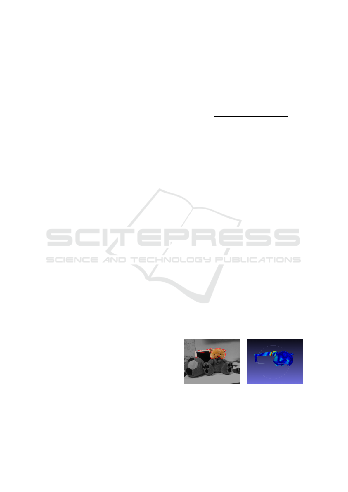
Figure 2: A 3D NURBS surface fitted over two clusters
originated by segmentation of the scene in Fig. 5, sixth row.
The red areas correspond to larger fit error. Notice how the
large fit error between the teddy head and the monitor por-
tion reveals that the two segments do not actually belong to
the same object. (Best viewed in color).
Joint Color and Depth Segmentation based on Region Merging and Surface Fitting
95

Once determined the (u
k
, v
l
) parameter values cor-
responding to the points to fit, the surface degrees and
the number of control points in the u, v parametric
directions, we consequently obtain the NURBS knots
(needed for the definition of the N
i,p
basis functions)
as in (Piegl and Tiller, 1997). Finally, by considering
Eq. (2) evaluated at (u
k
, v
l
) and equated to the points
to fit, we obtain an over-determined system of linear
equations. We solve it in the least-squares sense thus
obtaining the surface control points.
6 ITERATIVE REGION
MERGING PROCEDURE
The large number of segments produced by the ap-
proach of Section 4 needs to be combined into a
smaller number of segments representing the actual
objects and surfaces in the scene. The merging pro-
cedure follows the approach depicted in the right part
of Fig. 1 and summarized in Algorithm 1. Firstly a
NURBS surface is fitted on each segmented region
using the approach of Section 5. The fitting error cor-
responding to each segment S
i
is computed by eval-
uating the MSE value e
i
between the actual surface
points in the segment and the fitted NURBS surface.
Notice that other fitting accuracy measures besides
MSE can be considered, a complete review is pre-
sented in (Pagnutti and Zanuttigh, 2015). Then close
segments are analyzed in order to join segments with
similar properties.
The algorithm starts by sorting all the segments
based on decreasing fitting error e
i
thus producing an
ordered list L
S
where the segments with worse fitting
accuracy come first. The algorithm also analyzes all
the segments to build an adjacency matrix, storing for
each couple of segments whether they are adjacent or
not.
The following conditions must hold for two seg-
ments to be considered as adjacent:
1. They must be connected on the lattice defined by
the depth map (4-connectivity is used for this test)
and the length l
cc
of the shared boundary C
C
must
be bigger than 15 pixels.
2. The depth values on the shared boundary must be
similar. In order to perform this check for each
contour point C
i
we compute the difference ∆Z
i
between the depth values on the two sides of the
edge (see Fig. 3, the orange arrows underline
the differences that are computed). The number
of points l
d
cc
in the shared boundary which have
a depth difference smaller than a threshold T
d
is
then computed. The ratio between l
d
cc
and the to-
tal length of the shared boundary must be bigger
than a threshold R (the threshold is the same used
in Eq. (4) and (5) and we set it to 0.6), i.e.,:
|P
i
: (P
i
∈ C
C
) ∧ (∆Z
i
≤ T
d
)|
|P
i
: P
i
∈ C
C
|
=
l
d
cc
l
cc
> R
(3)
3. The color values must also be similar on both
sides of the common contour. The approach is the
same used for depth data except that the color dif-
ference in the CIELab is used instead of the depth
values. More in detail we compute the color dif-
ference ∆C
i
between samples on both side of the
shared boundary. The number of points l
c
cc
which
have a color difference smaller than threshold T
c
is computed and again the ratio between l
c
cc
and
the total length must be bigger than R, i.e.,
|P
i
: (P
i
∈ C
C
) ∧ (∆C
i
≤ T
c
)|
|P
i
: P
i
∈ C
C
|
=
l
c
cc
l
cc
> R
(4)
4. Finally the same condition is verified also for nor-
mal information. In this case the angle between
the two normal vectors ∆θ
i
is computed for each
couple of samples on the two sides of the shared
boundary. The number of points l
n
cc
which have
an angle between the normal vectors smaller than
T
θ
is computed and again the ratio between l
n
cc
and
the total length must be bigger than R, i.e.,
|P
i
: (P
i
∈ C
C
) ∧ (∆θ
i
≤ T
θ
)|
|P
i
: P
i
∈ C
C
|
=
l
n
cc
l
cc
> R
(5)
If all the conditions are satisfied the two segments are
marked as adjacent. Notice that by performing the
checks in the presented order we avoid unnecessary
computations, since we exclude most couple of seg-
ments before computing all the depth, color and nor-
mal differences on the contour.
The procedure then selects the segment with the
highest fitting error and tries to join it with the adja-
cent ones. Let us assume that we start from segment
Figure 3: Example of boundary region with the common
contour between two sample segments S
1
and S
2
and the
differences used in Equations (3), (4) and (5).
VISAPP 2016 - International Conference on Computer Vision Theory and Applications
96
46|P46 40|P40
58|P58 44,46
2
65|P65
30|P30 40,44,46
3
12|P12
24|P24
16|P16 4|P4
56,65
6
13|P13
33|P33
2|P2
14|P14
64|P64 13,40,44, 46
4
15|P15
57|P57
13,14,40, 44,46,61
7
8|P8
49|P49
17|P17
6|P6
8,29
8
18|P18
54|P54
17,20
9
19|P19 20|P20
19,31
10
21|P21
9
22|P22
21,26
11
23|P23
22,43
12
26|P26
23,27
13
27|P27
11
28|P28
13
29|P29 31|P31
8
32|P32
10
0|P0
19,31,32
14
34|P34
0,21,26
15
35|P35
34,58
1
36|P36
35,50
16
37|P37
10,36
17
38|P38
37,53
18
39|P39
38,41
19
1|P1 41|P41
1,22,43
20
42|P42
19
43|P43
42,45
21
44|P44
12
45|P45
2
3|P3
21
47|P47 48|P48 5|P5 50|P5 0
5,62
22
51|P51
16
52|P52 53|P53
13,14,25, 40,44,46,52 ,61
24
7|P7
18
55|P55
7,13,14,2 5,40,44,46,5 2,61
25
56|P56 25|P25
6
9|P9
13,14,25, 40,44,46,61
23
59|P59
9,11
26
60|P60 61|P61
7,13,14,2 5,37,40,44,4 6,52,53,56 ,60,61,63,65
35
62|P62
13,40,44, 46,61
5
63|P63
22
10|P10
56,63,65
27
11|P11
17 26
1
2,54
0 0
14
7,13,14,2 5,37,40,44,4 6,52,53,56 ,61,63,65
35
34
25
24
23
7
5
4
3
37,53,56, 63,65
34
32
32
27
0,1,8,9,10 ,11,17,20,2 1,22,23,26, 27,29,35,36 ,38,41,42,43 ,45,50
8,10,29,3 5,36,42,45,5 0
39
8,29,35,5 0
36
28 28
10,36,42, 45
36
3131
0,1,9,11,1 7,20,21,22, 23,26,27,38 ,41,43
39
0,21,23,2 6,27
38
30
30
15
1,9,11,17 ,20,22,38,41 ,43
38
9,11,17,2 0
37
29 29
1,22,38,4 1,43
37
33
33
20
Initial Segmentation Iteration 8 Iteration 16 Iteration 24 Iteration 32 Final Result
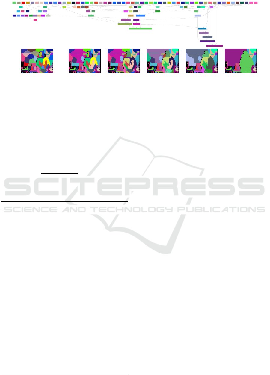
Figure 4: Example of the merging procedure on the scene of Fig. 5, fifth row. The images show the initial over-segmentation,
the merging output after 8,16,24 and 32 iterations and the final result (iteration 41). The graph shows the merge operations
between the various segments. The colors in the images correspond to those of the graph nodes. (Best viewed in color)
S
i
(the corresponding fitting error is e
i
): the algorithm
considers all the adjacent segments S
j
(with fitting er-
ror e
j
) and fits a NURBS surface on each segment
obtained by joining S
i
and each of the S
j
(let us de-
note it with S
i∪ j
). The fitting error e
i∪ j
on segment
S
i∪ j
is computed with the same previous method and
compared with the weighted average of the errors on
S
i
and S
j
:
e
i
|S
i
| + e
j
|S
j
|
e
i∪ j
(|S
i
| + |S
j
|)
> 1 (6)
If the condition of Eq. (6) is satisfied the two
segments are candidate to be merged, since the fit-
Algorithm 1: Merge algorithm.
Compute L
S
(list of the segments) and sort the list
according to e
i
For each segment S
i
compute the set A
i
of the adja-
cent segments
i = 1 (select as S
i
the first segment in L
S
)
while i < length(L
S
) do
for all the segments S
j
adjacent to S
i
do
compute the fitting error on the merged seg-
ment S
i∪ j
check if the threshold of Eq. 6 is satisfied
end for
if there is at least one merge operation satisfying
Eq. 6 then
Select the merge leading to the biggest fitting
accuracy decrease (the corresponding segment
is S
∗
j
)
Remove S
i
and S
∗
j
from L
S
Add S
i∪ j
∗
to L
S
Compute A
i∪ j
∗
i = 1 ( S
i
is the first segment in L
S
)
else
i = i + 1 (S
i
is the next segment in the list)
end if
end while
ting accuracy is improved for their union. The pro-
cedure is repeated for all the segments adjacent to S
i
.
If more than one segment S
j
is selected as candidate
for the merge operation, the segment S
∗
j
that provides
the maximum improvement of the fitting error accord-
ing to Eq. (6) is selected. If there are no candidates
no merge operation is performed, the algorithm se-
lects the next one in the sorted list as new segment
S
i
and the procedure is repeated. Otherwise the two
segments S
i
and S
∗
j
are joined and their union S
i∪ j
∗
replaces them in the list L
S
. The adjacency informa-
tion is then updated by considering the union of S
i
and S
∗
j
as adjacent to all the segments that were ad-
jacent to any of the two segments, and the list L
S
is
updated by removing the two joined segments and in-
serting their union in the position corresponding to its
fitting error e
i∪ j
∗
. The algorithm continues by pro-
cessing the next segment with the highest fitting error
and iterates until no more segments can be consid-
ered for the merge operation. The procedure is sum-
marized in Algorithm 1 and its progress on a sam-
ple scene is visualized in Fig. 4 where a graph of
the merge operations between the various segments
and the resulting segmentations at various iterations
are shown. The sequence of merging steps on var-
ious scenes is also shown in the videos available at
http://lttm.dei.unipd.it/downloads/segmentation.
7 EXPERIMENTAL RESULTS
The performances of the proposed method
have been evaluated on two different datasets.
The first dataset is available at http://lttm.dei.
unipd.it/downloads/segmentation and contains 6
different images and depth maps of some sample
scenes.
The scenes have been segmented with the pro-
Joint Color and Depth Segmentation based on Region Merging and Surface Fitting
97
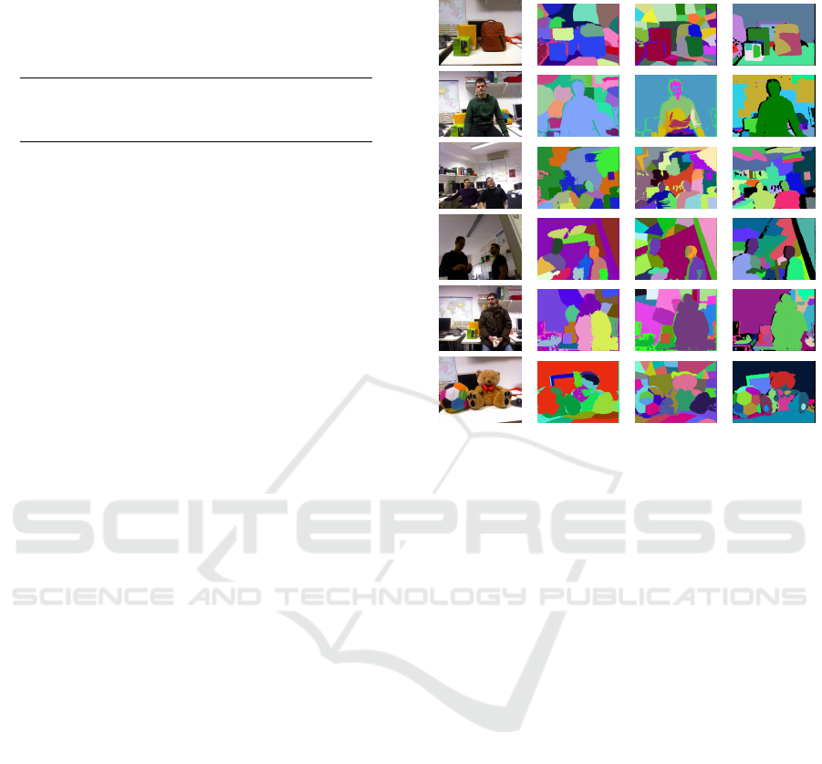
Table 1: Comparison of the performances of the proposed
method with (Dal Mutto et al., 2012a) and (Pagnutti and
Zanuttigh, 2014). The table shows the average value of the
VoI and RI metrics on the six scenes of the dataset made
available by the authors of (Pagnutti and Zanuttigh, 2014).
Approach VoI RI
(Dal Mutto et al., 2012a) 2.56 0.84
(Pagnutti and Zanuttigh, 2014) 2.69 0.83
Proposed Method 1.69 0.90
posed method and the obtained results are shown in
Fig. 5 while Table 1 presents the numerical results
obtained by comparing the data with a manually seg-
mented ground truth. The figure and table also present
a comparison with two competing approaches.
Starting from visual results, Fig. 5 compares the
proposed approach with the methods of (Dal Mutto
et al., 2012a), that directly segments the image into
the desired number of regions with an approach based
on spectral clustering (it can be considered a sim-
plified version of the initial segmentation scheme of
Sec. 4) and of (Pagnutti and Zanuttigh, 2014) that ex-
ploits a region splitting scheme that recursively parti-
tions each segmented region in two parts. It clearly
obtains better performances than the compared ap-
proaches. In fact the region merging scheme allows
to avoid the creation of small clusters due to noise or
objects with a complex surface and at the same time to
properly extract the main objects in the scene. Notice
that the compared approaches are not able to properly
segment into a single region some very large objects
(e.g., the background in rows 1 and 5 or the people
in row 3) since the geometrical component forces the
division of them into several pieces. The bias towards
segments of similar size is a known issue of the nor-
malized cuts algorithm and of the derived approaches,
but the proposed merging scheme solves this problem
by recombining together segments belonging to the
same surface. The use of orientation information al-
lows to properly recognize the various walls and sur-
faces with different orientation unlike the compared
approaches (e.g., the table in the first row or the back-
ground in row 3). In general the objects are well rec-
ognized and there are almost no segments extending
over multiple objects at different depths. The edges
of the objects are also well captured and there are no
small thin segments extending along the edges as for
some other schemes.
The visual evaluation is confirmed by numer-
ical results, as shown by Table 1 (additional
data are available at http://lttm.dei.unipd.it/down
loads/segmentation). In order to compare the ob-
tained results with ground truth data we used two dif-
ferent metrics, i.e., the Variation of Information (VoI)
Color Dal Mutto Pagnutti Proposed
Image et Al. et Al. Method
Figure 5: Segmentation of some sample scenes with the
proposed method and with the approaches of (Dal Mutto
et al., 2012a) and of (Pagnutti and Zanuttigh, 2014). The
black regions for the proposed approach correspond to sam-
ples without a valid depth value from the Kinect that have
not been considered for the segmentation.
and the Rand Index (RI). A description of these error
metrics can be found in (Arbelaez et al., 2011), notice
in particular that a lower value corresponds to a better
result for the VoI metric while a higher value is better
for the RI metric. The table shows the average val-
ues of the 2 metrics on the six considered scenes. It
shows how the proposed approach outperforms both
the compared ones. The VoI metric value is better by
a large gap, with an average of 1.69 against 2.56 and
2.69, and also the RI metric gives a better result with
an average value of 0.9 against 0.84 and 0.83 achieved
by the two competing approaches.
The second considered dataset is the much larger
NYU Depth Dataset V2 (Silberman et al., 2012). This
dataset has been acquired with the Kinect and con-
tains 1449 depth and color frames from a variety of
indoor scenes. For the numerical evaluation we used
the updated versions of the ground truth labels pro-
vided by the authors of (Gupta et al., 2013). Ta-
ble 2 shows the comparison between our approach
and some competing schemes on this dataset (for the
other approaches we collected the results from (Has-
nat et al., 2014) ). The compared approaches are
the clustering and region merging method of (Hasnat
et al., 2014), the MRF scene labeling scheme of (Ren
VISAPP 2016 - International Conference on Computer Vision Theory and Applications
98
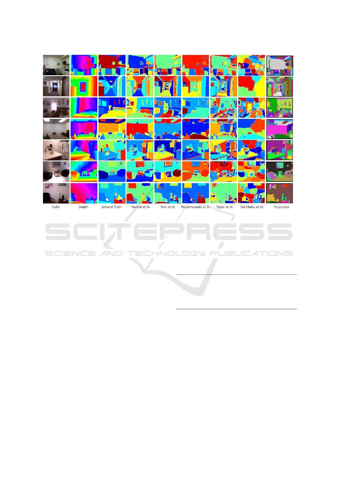
Figure 6: Segmentation of some sample scenes from the NYUv2 dataset: (column 1) color data; (column 2) depth data;
(column 3) ground truth; (column 4) (Hasnat et al., 2014); (column 5) (Ren et al., 2012); (column 6) (Felzenszwalb and
Huttenlocher, 2004); (column 7) (Taylor and Cowley, 2013); (column 8) (Dal Mutto et al., 2012a); (column 9) proposed
method. The results for the competing methods have been collected from (Hasnat et al., 2014).
et al., 2012), a modified version of (Felzenszwalb and
Huttenlocher, 2004) that accounts also for geome-
try information, the dynamic programming scheme of
(Taylor and Cowley, 2013) and the clustering-based
approach of (Dal Mutto et al., 2012a). The average
values obtained by our method are 2.23 according to
the VoI metric and 0.88 according to RI. The results
according to VoI show that our approach outperforms
all the compared ones. If the RI metric is consid-
ered instead, the proposed method outperforms the
schemes of (Felzenszwalb and Huttenlocher, 2004),
(Taylor and Cowley, 2013) and (Dal Mutto et al.,
2012a) and obtains results almost identical to those
of the very recent state-of-the-art methods of (Hasnat
et al., 2014) and (Ren et al., 2012) with a negligible
difference of 0.02. Notice also that our approach does
not make any assumption about the presence of planar
surfaces in the scene as done by (Hasnat et al., 2014)
and (Taylor and Cowley, 2013), so it better general-
izes to scenes with non-planar surfaces (in the NYUv2
dataset all the scenes are indoor settings with a lot of
planar surfaces like walls and furniture, but outdoor
settings have a large variability). In addition the ap-
proach of (Ren et al., 2012) exploits a learning stage
on the NYU dataset, while our approach does not as-
sume any previous knowledge on the data.
Table 2: Comparison of the performances of the proposed
method with some state-of-the-art approaches. The table
shows the average value of the VoI and RI metrics on the
1449 scenes of the NYUv2 dataset.
Approach VoI RI
(Hasnat et al., 2014) 2.29 0.90
(Ren et al., 2012) 2.35 0.90
(Felzenszwalb and Huttenlocher, 2004) 2.32 0.81
(Taylor and Cowley, 2013) 3.15 0.85
(Dal Mutto et al., 2012a) 3.09 0.84
Proposed Method 2.23 0.88
A visual comparison on 7 different scenes from
this dataset is shown in Fig. 6 (notice that the scenes
have been selected by the authors of (Hasnat et al.,
2014)). Even if this dataset is more challenging, the
proposed approach is able to obtain a reliable segmen-
tation on all the considered scenes and visual results
confirm the numerical ones. The obtained segmenta-
tions are much better than the approaches of (Felzen-
szwalb and Huttenlocher, 2004), (Dal Mutto et al.,
2012a) and (Taylor and Cowley, 2013) (columns 6-7-
8) on the considered scenes. The comparison with the
two best performing approaches, i.e., (Hasnat et al.,
2014) and (Ren et al., 2012), is more challenging but
the proposed scheme is able to outperform them on
Joint Color and Depth Segmentation based on Region Merging and Surface Fitting
99

various scenes. In particular our approach produces
quite clear edges with no noisy small segments in
their proximity, an issue happening with other ap-
proaches on some scenes. Foreground objects are also
clearly extracted and the background region is cor-
rectly handled on most scenes. However some small
issues are present in the corridor and bed scenes (rows
2 and 3). In particular the blanket of the bed scene
(row 3) is quite critical for our approach since the
color data is very noisy and the orientation of the nor-
mals on the rough surface is very unstable.
8 CONCLUSIONS
In this paper we have introduced a novel scheme for
the joint segmentation of color and depth informa-
tion. The proposed approach exploits together spatial
constraints, surface orientation information and color
data to improve the segmentation performances. The
regions of the initial over-segmentation are merged
by exploiting a surface fitting scheme that allows to
determine if the regions candidate for merging cor-
respond to the same 3D surface. Experimental re-
sults demonstrate the effectiveness of this scheme
and its ability to recognize the objects in the scene.
Performances on real data acquired with the Kinect
show that the proposed method is able to outperform
state-of-the-art approaches in most situations. Fur-
ther research will be devoted to the combination of
the proposed approach with a recursive region split-
ting scheme. Furthermore, an advanced scheme for
the automatic balancing of the various clues relevance
will be developed. Finally, since our region merging
algorithm is highly vectorizable, parallel computing
implementations will be considered.
REFERENCES
Arbelaez, P., Maire, M., Fowlkes, C., and Malik, J. (2011).
Contour detection and hierarchical image segmenta-
tion. Pattern Analysis and Machine Intelligence, IEEE
Transactions on, 33(5):898–916.
Bleiweiss, A. and Werman, M. (2009). Fusing time-of-
flight depth and color for real-time segmentation and
tracking. In Proc. of DAGM Workshop, pages 58–69.
Dal Mutto, C., Zanuttigh, P., and Cortelazzo, G. (2011).
Scene segmentation assisted by stereo vision. In Pro-
ceedings of 3DIMPVT 2011, Hangzhou, China.
Dal Mutto, C., Zanuttigh, P., and Cortelazzo, G. (2012a).
Fusion of geometry and color information for scene
segmentation. IEEE Journal of Selected Topics in Sig-
nal Processing, 6(5):505–521.
Dal Mutto, C., Zanuttigh, P., and Cortelazzo, G. M.
(2012b). Time-of-Flight Cameras and Microsoft
Kinect. SpringerBriefs. Springer.
Erdogan, C., Paluri, M., and Dellaert, F. (2012). Planar
segmentation of rgbd images using fast linear fitting
and markov chain monte carlo. In Proc. of CRV.
Felzenszwalb, P. and Huttenlocher, D. (2004). Efficient
graph-based image segmentation. International Jour-
nal of Computer Vision, 59(2):167–181.
Fowlkes, C., Belongie, S., Chung, F., and Malik, J. (2004).
Spectral grouping using the nystr
¨
om method. IEEE
Transactions on Pattern Analysis and Machine Intel-
ligence, 26(2):214–225.
Gupta, S., Arbel
´
aez, P., Girshick, R., and Malik, J.
(2014). Indoor scene understanding with rgb-d im-
ages: Bottom-up segmentation, object detection and
semantic segmentation. International Journal of Com-
puter Vision, pages 1–17.
Gupta, S., Arbelaez, P., and Malik, J. (2013). Perceptual
organization and recognition of indoor scenes from
RGB-D images. In Proceedings of CVPR.
Hasnat, M. A., Alata, O., and Trmeau, A. (2014). Unsuper-
vised rgb-d image segmentation using joint clustering
and region merging. In Proceedings of BMVC.
Pagnutti, G. and Zanuttigh, P. (2014). Scene segmentation
from depth and color data driven by surface fitting. In
IEEE International Conference on Image Processing
(ICIP), pages 4407–4411. IEEE.
Pagnutti, G. and Zanuttigh, P. (2015). Scene segmentation
based on nurbs surface fitting metrics. In In proc. of
STAG Workshop.
Piegl, L. and Tiller, W. (1997). The NURBS Book (2Nd Ed.).
Springer-Verlag, Inc., New York, USA.
Ren, X., Bo, L., and Fox, D. (2012). Rgb-(d) scene labeling:
Features and algorithms. In Proc. of CVPR.
Shi, J. and Malik, J. (2000). Normalized cuts and image
segmentation. IEEE Transactions on Pattern Analysis
and Machine Intelligence, 22(8):888–905.
Silberman, N., Hoiem, D., Kohli, P., and Fergus, R. (2012).
Indoor segmentation and support inference from rgbd
images. In Proceedings of ECCV.
Srinivasan, N. and Dellaert, F. (2014). A rao-blackwellized
mcmc algorithm for recovering piecewise planar 3d
model from multiple view rgbd images. In IEEE In-
ternational Conference on Image Processing (ICIP).
Taylor, C. J. and Cowley, A. (2013). Parsing indoor scenes
using rgb-d imagery. In Robotics: Science and Sys-
tems, volume 8, pages 401–408.
Wallenberg, M., Felsberg, M., Forss
´
en, P.-E., and Dellen,
B. (2011). Channel coding for joint colour and depth
segmentation. In Proc. of DAGM, volume 6835, pages
306–315.
VISAPP 2016 - International Conference on Computer Vision Theory and Applications
100
