Sensor Localization using Signal Receiving Probability

and Procrustes Analysis

Ashanie Gunathillake

1,2

, Andrey V. Savkin

, Anura Jayasumana

and Aruna Seneviratne

1,2

School of Electrical Engineering and Telecommunication, University of New South Wales, Sydney NSW 2052, Australia

NICTA, Eveleigh, NSW 2015, Australia

Department of Electrical and Computer Engineering, Colorado State University, Fort Collins, CO 80523, U.S.A.

Keywords:

Localization, Procrustes Analysis, Signal Propagation, Wireless Sensor Network.

Abstract:

The location information of sensors is of great importance for wireless sensor network automation and has

been one of the major challenges in large-scale sensor networks. In order to improve the localization accuracy

of sensors, the gain of both range-free and range-based approaches need to be concerned. In this paper,

we propose a new localization algorithm based on signal receiving probability and Procrustes analysis. A

critical observation in range-free technique is sensors can move a non-zero distance without changing it’s

connectivity information. To defeat that difﬁculty and achieve a better ranging measurement, a receiving

probability function, which is sensitive to the distance, is used in this paper. The probability function is used

to calculate the topological coordinates and then to transform it to physical coordinates, the Procrustes analysis

is used. The result shows that our proposed algorithm has been able to calculate the physical coordinates of

sensors, which are distributed over an area, consist of obstacles and with different environmental conditions.

Moreover, it outperformed the other existing algorithms by a maximum localization error less then 2m.

1 INTRODUCTION

Wireless Sensor Networks (WSNs) applications cover

a large number of domains spanning environmen-

tal monitoring, military, agriculture, transportation

and inventory tracking (Garca-Hernndez et al., 2007)

(Tubaishat and Madria, 2003). Future WSNs will be

large-scale networks automated to self-organized and

perform a speciﬁc task. Thus, the location map of the

sensors is required.

However, ﬁnding the locations of the sensors is

crucial and has received substantive attention in re-

cent years. The algorithms used to calculate the

physical coordinates of the sensors can be divided

into two categories, namely Range-based and Range-

free localization algorithms. Range-based algorithms

use special hardware component to measure range-

based parameters such as received signal strength

(RSS) (Chengdong et al., 2011), time of arrival(TOA)

(Wang and Ho, 2013), angle of arrival (AOA) (Kotwal

et al., 2010). These algorithms are affected by noise,

fading and interference, and as a result, their accuracy

decreases in environments with obstacles. Range-free

algorithms rely on the information about the connec-

tivity of the sensors instead of using special hardware

device. However, the accuracy of the algorithms is

highly depended on the number of anchor nodes i.e.

nodes known their locations, and their distribution.

To this end, we are proposing a localization algo-

rithm based on Receiving Probability and Procrustes

Analysis (RP-PA). Here we are trying to achieve the

advantages in both range-based and range-free tech-

niques. As in range-free algorithms we do not use

any special hardware component, but to calculate the

distances, a signal receiving probability function that

is sensitive to the distance is used. Since we are not

using any hardware component to measure the dis-

tances, the hardware cost of the network can mini-

mize.

RP-PA algorithm uses a receiving signal probabil-

ity function to reduce the dependency on range-based

measurements. It starts from ﬁnding the topology

map of the network using the probability function.

Topology map is an arrangement of nodes without af-

fecting it’s connectivity information. In RSSI based

algorithms, the distances are extracted from receiv-

ing power that encounters some error due to RF com-

munication effects. Thus, we evaluate the connectiv-

ity information without taking those error prone pa-

rameters. In range-free algorithms, they consider the

Gunathillake, A., Savkin, A., Jayasumana, A. and Seneviratne, A.

Sensor Localization using Signal Receiving Probability and Procrustes Analysis.

DOI: 10.5220/0005671301130120

In Proceedings of the 5th International Confererence on Sensor Networks (SENSORNETS 2016), pages 113-120

ISBN: 978-989-758-169-4

113

connectivity information with the hop counts to the

anchor nodes, but it is not sensitive to the distance.

As a result, it is possible to move a sensor node over

a non-zero distance without changing the hop count.

Hence, range-free algorithms generate physical coor-

dinates with less accuracy. To overcome this problem,

we construct the connectivity information matrix us-

ing a probability function, which is sensitive to the

distance between sensor nodes.

To transform the topology coordinates to physical

coordinates, the algorithm uses the Procrustes Analy-

sis. From the result, it can be seen that the proposed

RP-PA algorithm is able to provide accurate physical

coordinates of the sensors. Also, it results in an error

less than 2m and outperforms the RSSI and hop-based

localization algorithms.

2 BACKGROUND

Prior work on localization techniques, can be grouped

into two categories range-based and range-free local-

ization. In range-based techniques special hardware

device is used to measure the range-based parameters

such as signal strength, time of arrival and angle of

arrival. In received signal strength indicator (RSSI)

based localization algorithms, signal strength of re-

ceiving packets is used to estimate the distance be-

tween nodes. The distance calculation of these algo-

rithms use two models namely, theoretical and em-

pirical models (Zhang et al., 2012). In theoretical

models, RF signal transmission loss model is used

to directly calculate the distance between two nodes

(Mukhopadhyay et al., 2014)(Al Alawi, 2011). The

empirical models, use a two steps process to ob-

tain the location. First, they create an ofﬂine RSSI

database, using anchor nodes. Secondly, it determines

the coordinates of non-anchor nodes by matching the

received signal strength to a record of the database

(Chengdong et al., 2011)(Wanga et al., 2011).

The localization method based on time difference

of arrival (TDOA) estimates the coordinates of an un-

known node by anchor nodes’ coordinates and time

difference of arrival from those anchors to the node.

For the calculation, it needs at least four anchors

(Savarese et al., 2002) (Luo et al., 2012) (Liu et al.,

2012) (Wang and Ho, 2013) (Huang et al., 2015).

Furthermore, in time of arrival (TOA) based local-

ization, the anchor nodes broadcast a signal and the

sensor nodes that receive these broadcasts, use the

time difference of arrival , RSS and a the angle of

arrival to determine their locations. This requires

the sensor timers have to be synchronized. To over-

come this requirement, researchers have proposed the

use of Round-Trip TOA (RTOA) (Wymeersch et al.,

2009) and Two Way TOA (TW-TOA) (Gholami et al.,

2012)(Oguz-Ekimet al., 2013). Again, TOA localiza-

tion does not address issues associated with obstacles

and RF signal transmission affects.

In range-free localization algorithms, the loca-

tions of nodes are obtained without using any spe-

cial hardware. They rely on the connectivity infor-

mation of nodes. First, it gets the distance in hops

and then maps the hop distance to geometric distance

(Niculescu and Nath, 2003)(Tian et al., 2003)(Liu

et al., 2004) using anchor node locations. Therefore,

the accuracy of these algorithms highly depends on

the number of anchor nodes and their deployment.

The key issue of range-free algorithms is the distance

estimation i.e. the mapping of the hop distance to ge-

ometric distance.

Dulanjalie et al. (Dhanapala and Jayasumana,

2014) presented a method to obtain topology-

preserving maps of WSNs using virtual coordinates

(VCs) of sensor nodes. Topological mapping tech-

niques are fundamentally different to localization

techniques because the mapping algorithms are con-

cerned with the arrangement of the nodes. They are

not concerned about the actual location of the nodes.

In other words, the mapping schemes expect the rel-

ative distances to be accurate, not the physical dis-

tances. Thus, given the absolute position of a subset

of nodes, global localization is realizable. However,

to achieve this, the topological map should be isomor-

phic to the physical layout of the sensor network. In

Virtual Coordinate System (VCS), the layout infor-

mation such as physical voids, shape, and etc. are

absent. Furthermore, Dulanjalie et al.(Dhanapala and

Jayasumana, 2014) have shown that transformation

for topological map from virtual coordinates can be

generated using a subset of nodes. However, when the

number of nodes increase, the time required to gener-

ate the virtual coordinate matrix also increases.

3 DETAILS OF THE PROPOSED

ALGORITHM: RP-PA

This section describes the work ﬂow of RP-PA algo-

rithm, that calculates the physical coordinates of the

sensors. The physical map is achieved by using the

packet receiving probability function and Procrustes

transformation. RP-PA algorithm consider two as-

pects i.e. accuracy of range measurements and the

accuracy of the coordinate. The range measurement

accuracy is obtained by the receiving signal proba-

bility function sensitive for the distance. First using

the probability values, the topological coordinates of

SENSORNETS 2016 - 5th International Conference on Sensor Networks

114

each node is calculated. Then to achieve the local-

ization accuracy, Procrustes analysis is carried out in

each node. The detail of the algorithm is described in

following subsection.

3.1 Topological Coordinates

The ﬁrst task of the RP-PA algorithm is to calculate

the coordinate of nodes in topological map. Topol-

ogy map represents the arrangement of nodes without

affecting the connectivity information of nodes. To

ﬁnd the connectivity information, receiving probabil-

ity function, which describes below, is used.

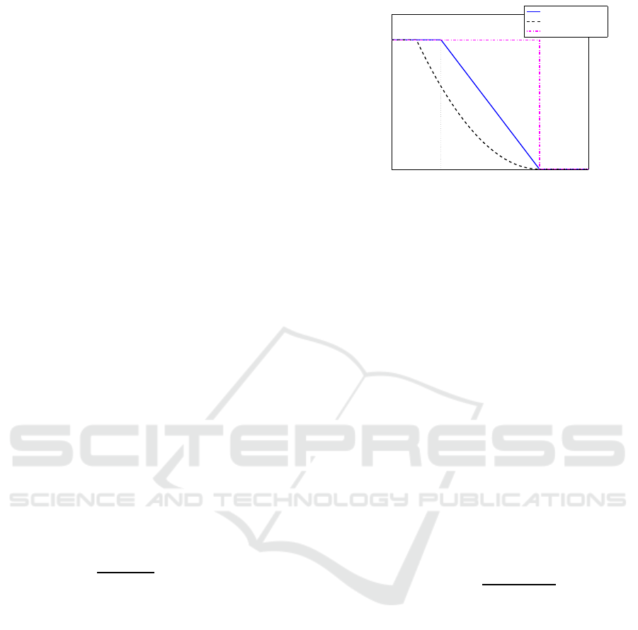
3.1.1 The Receiving Probability Function

This function describes the probability of packet re-

ceiving from sensor when anchor node is located at a

particular distance. Let, S(d) be the probability value

when anchor node is at distance d from the sensor.

Then, S(d) satisﬁes the following constraints:

0 ≤ S(d) ≤ 1 ∀d

S(d

) ≤ S(d

) ∀d

≥ d

S(d) = 0 ∀d > R (1)

where R > 0 is some given distance.

Such a function S(d) is called the receiving prob-

ability function. We will use the following example

of such a function:

S(d) := p

∀d ≤ r

S(d) := 0 ∀d ≥ R

S(d) :=

(R− d)

(R− r)

∀r < d < R (2)

where 0 < p0 ≤ 1, 0 < r < R < R

are some given

constants. R

is the communication range of a sensor

node. It is obvious that the function (2) satisﬁes all

the conditions (1).

The receiving probability function we are using

is an intermediate model of RSSI signal receiving

and hop-based packet receiving. As shown in Fig-

ure 1, it can be seen that hop based algorithms use the

r = R assumption, which cannot be achieved in real

environment. On the other hand, RSSI localization

uses a polynomial function to estimate packet receiv-

ing probability, which is hard to estimate the parame-

ters for different environmental situations. Therefore,

here we consider an intermediate level between RSSI

model and VC model to obtained the topological co-

ordinates.

Distance

Packet receiving probability

Linear decay model

RSSI model

VC model

Figure 1: Packet receiving probability function for different

models.

3.1.2 Calculating Topological Coordinates

This section describes the topological coordinate cal-

culation using the receiving probability function. Let

consider a network consist with N number of steady

sensors in unknown locations labeled i = 1, 2,..., N

and M(< N) number of steady anchor nodes that

know their locations labeled A

, j = 1, 2...M. The an-

chor nodes transmit signals at times t

< t

< ... < t

to it’s one-hop neighborhood. We introduce a binary

matrix M

of order a× S by the following rule. Here,

a is the number of anchor nodes in node i’s neighbor-

hood.

( j, s) = 1, if node i gets a signal from the anchor A

at the time t

;

( j, s) = 0, if node i does not get a signal from the

anchor A

at the time t

Then, based on the M

matrix, signal receiving

probability matrix RP

of order a× 1is deduced as fol-

lows.

( j, 1) =

∑

s=1

( j, s)

(3)

Finally, based on the anchor node positions,

the receiving probability function S(d) and the

receiving probability matrix RP

, we obtain the

topological coordinates of the sensors. Let

(1, 1), AP

(2, 1), ..., AP

(a, 1) denote the elements

of the vector AP

. Furthermore, the probability for

a sensor node to receive a signal from a anchor

node A

is described by the function S(d) where d

is the distance between the anchor and the sensor

node i at the time of sending the signal. Thus we

can map the probability values to a distance vector

using the receiving probability function denoted as

(1, 1), d

(2, 1)...d

(a, 1) respectively.

After knowing the distance of the vector of sen-

sor i, we have used trilateration to calculate the co-

ordinate of the node with respect to the anchors

in its ﬁrst hop neighborhood. The coordinates of

the anchors in node i’s ﬁrst hop neighborhood are

Sensor Localization using Signal Receiving Probability and Procrustes Analysis

115

0 5 10 15 20 25 30

(a)

Localization Error

(b)

0 5 10 15 20 25 30

(c)

Localization Error

(d)

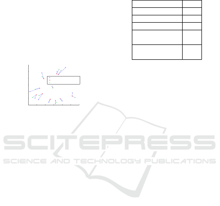
Figure 2: (a) Circular-shaped network, (b) Error distribution, (c) Concave void network and (d) Error distribution.

, y

), (x

, y

)...(x

, y

). The topological coordinate

of the node i is (x

, y

) is given by the equation 4.

= B (4)

where,

A =







− x

) 2y

− y

)

− x

) 2y

− y

)

− x

a−1

) 2y

− y

a−1

)











and

B =







− x

) + (y

− y

) + (d

(a, 1) − d

(1, 1))

− x

(

a− 1)

) + (y

− y

(

a− 1)

(a, 1) − d

(1, 1))







To ﬁnd an optimal topological coordinates of the

sensors, we used the Least square approximation.

Here the objective function is given as in condition 6

and by solving to X

∗t

we got the solution as in equa-

tion .

Min k AX

∗t

B k

(5)

∗

= (AA)

−1

(A)B (6)

where, X

∗

= [x

∗t

]

3.2 Obtaining Physical Coordinates

using Procrustes Analysis

This section describes the transformation of topolog-

ical coordinates to physical coordinates using Pro-

crustes analysis. Procrustes Analysis is used to align

two sets of data points. Here we used it to obtain

physical coordinate of sensors from the topological

coordinates that is calculated in the previous section.

Procrustes analysis calculates the scaling factor,

rotation angle and shift between the two sets (Nhat

et al., 2008). If the transformation between the two

sets is not linear, Procrustes analysis will ﬁnd the

transformation which has an error. Thus we need

to make sure that topological coordinates have lin-

earized error with the actual sensor location. Figure

2 shows the error distribution of the topological co-

ordinates with respect to the actual positions of the

sensor nodes. According to the ﬁgure, the error dis-

tribution is not linear for the whole network. Hence, a

single transformation can not be applied to the whole

network.

To overcome that problem, transformation factors

are calculated in each node based on it’s one hop an-

chor nodes. Let consider sensor node i have a number

of anchor nodes in it’s ﬁrst hop neighborhood. Then

X and Y are the topological and physical coordinate

matrices with length of a × 2 respectively. Thus the

transformation factors of node i can be estimated by

equation 7.

SENSORNETS 2016 - 5th International Conference on Sensor Networks

116

Y = bXT + c; (7)

where b is the scaling factor, T is the rotation an-

gle and c is the shift value. When the transformation

factors are estimated, node i can calculates it’s phys-

ical coordinates using the equation 7 where X is the

topological coordinates of node i and Y is the physical

coordinates of node i. Figure 3 compares the localiza-

tion error before and after the Procrustes analysis. In

this experiment, we can see that each node uses a dif-

ferent transformation factor to calculates it’s physical

coordinates. Thus the localization error has been re-

duced.

0 5 10 15 20 25 30

Actual Position

Topological Coordinates

Calculated Physical Coordinates

Figure 3: Impact of Procrustes Analysis.

4 RESULT

The performance of the proposed RP-PA algorithm

is evaluated in this section. First the receive signal

strength model used for the simulation is described.

Then the performance of the algorithm is compared

with other existing algorithms. MATLAB simulation

software was used for the computations.

4.1 Receive Signal Strength Model

The received signal strength can be modeled as hav-

ing two components such as path loss and shadow-

ing (Pathirana et al., 2005). Therefore, the commonly

used propagation model of RF signals is given in

equation (8).

rx,i

(t) = P

tx, j

− 10εlogd

(t) + v

(t) (8)

where, the received signal strength at node i at

time t is P

rx,i

(t), the transmitted signal strength of the

signal at node j is P

tx, j

, the path-loss exponent is ε,

the distance between node i and node j at time t is

(t) and the logarithm of shadowing component on

node i at time t is v

(t).

However, this model is not suitable for a network

with some obstacles. In (Lott and Forkel, 2001), they

proposed a MultiWall-Multiﬂoor Model for RF com-

munication. In this model the variation of the absorp-

tion against the thickness of the medium which signal

Table 1: Simulation Parameters.

Parameter Value

Transmitted power -50dB

Sensitivity -90dB

Communication radius 10m

Suburban area ε = 2.7

σ =9.6

Light tree density area ε = 3.6

σ =8.2

traverse, is not considered. Therefore we updated the

equation (8) by using the Lambert-Bouguer law. Let

ob,i

(t) is the loss due to signal absorption from ob-

stacles exist in the line of sight of node i and j at time

t, then the RF signal propagation model is as in equa-

tion (9).

rx,i

(t) = P

tx, j

− 10εlogd

(t) − L

ob,i

(t) + v

(t) (9)

The absorption coefﬁcient and the thickness of the

obstacle medium, which signal traverses are α and

(t) respectively. Then L

ob,i

(t) can be calculated as,

ob,i

(t) = Σ

k=1

10αd

(t)log(e) (10)

where, n is the number of obstacles exist in between

node i and node j.

4.2 Performance Evaluation

The performance of the receiving probability ap-

proach and other two localization approaches, that

are RSSI based(Mukhopadhyay et al., 2014) and hop

based (Dhanapala and Jayasumana, 2014), is evalu-

ated through large-scale simulations. To make the ca-

parison equitable for all three approaches, the Pro-

crustes analysis is applied to each output obtained

from the above three approaches.

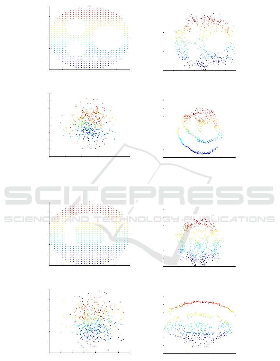
The large-scale WSNs we selected for the evalua-

tion is shown in Figure 4 and 5 . Here we have dif-

ferent shapes of networks with obstacles. The Figure

4(a) is a 496 sensor nodes circular-shaped network in

a suburban area with three physical obstacles (con-

crete barriers). The Figure 5(a) is a 554 sensor nodes

network with a concave void (concrete barriers) in a

light tree density area. Table 1 presents the simula-

tion parameters. Here we consider anchor nodes are

randomly distributed over the network area.

Figure 4 and 5, clearly demonstrate the effective-

ness of the proposed algorithm. However to compare

the performance of the algorithm, we calculate the lo-

calization error as in the equation 11. Figure 6 com-

Sensor Localization using Signal Receiving Probability and Procrustes Analysis

117

0 5 10 15 20 25 30

(a)

−5 0 5 10 15 20 25 30

(b)

−10 0 10 20 30 40

−5

(c)

−10 0 10 20 30 40

(d)

Figure 4: (a) Circular-shaped network with 496 nodes , (b) Output of proposed RP-PA algorithm, (c) Output of RSSI algorithm

and (d) Output of Hop based algorithm.

0 5 10 15 20 25 30

(a)

−10 0 10 20 30 40

(b)

−5 0 5 10 15 20 25 30

(c)

0 5 10 15 20 25 30

−5

(d)

Figure 5: (a) Circular-shaped concave void network with 554 nodes , (b) Output of proposed RP-PA algorithm, (c) Output of

RSSI algorithm and (d) Output of Hop based algorithm.

SENSORNETS 2016 - 5th International Conference on Sensor Networks

118

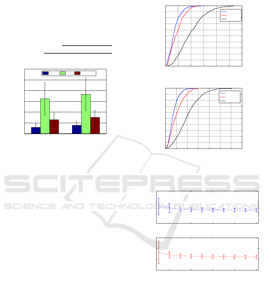
pares the localization error of the three methods men-

tioned above for the two network distributions. It can

be seen that the proposed RP-PA algorithms outper-

forms the other two methods by having a average lo-

calization error less than 2m.

location

rror =

∑

i=1

− x

)

+ (y

− y

)

(11)

Figure 4 Figure 5

Localization Error

RP−PA RSSI Hop−count

Figure 6: Localization error comparison.

Moreover, to analyze the localization error more

enormously, Figure 7 compares the cumulative distri-

bution of the localization error of three methods for

the two networks. From Figure 7(a) and Figure 7(b),

it can be seen that 80% of nodes have less than 2m

localization error with RP-PA algorithm. Hence it is

seen that RP-PA algorithm performs better than RSSI

and hop based localization algorithms.

Figure 8 shows the performance of the RP-PA al-

gorithm against the number of anchor nodes. Accord-

ing to the ﬁgure, RP-PA algorithm has been able to

generate physical coordinates of sensor nodes with

less than 2m average localization error for the two net-

work deployed in different environmental situations

using 10% of anchor nodes. Thus, with less amount

of sensor nodes, the algorithm can calculate the loca-

tion of sensors in a large-scale WSN.

5 CONCLUSION

We presented a RP-PA algorithm, which calculates

the coordinates of sensor nodes without using any

special hardware component. RP-PA algorithm ex-

tracts the advantages if range-based and range-free

localization techniques. In range-free approach, the

connectivity information is obtained by hop-count

matrix and as a result sensors can move non-zero dis-

tance without affecting the connectivity information.

However in range-based algorithms, RF communi-

cation effects such as noise, fading and interference

0 2 4 6 8 10 12

0.1

0.2

0.3

0.4

0.5

0.6

0.7

0.8

0.9

Localization Error %

CDF of Localization Error

Empirical CDF

RP−PA

Hop−count

RSSI

(a)

0 2 4 6 8 10 12 14

0.1

0.2

0.3

0.4

0.5

0.6

0.7

0.8

0.9

Localization Error %

CDF of Localization Error

Empirical CDF

RP−PA

Hop−count

RSSI

(b)

Figure 7: (a) CDF of localization error in Figure 4 network,

(b) CDF of localizatio error in Figure 5 network.

10 20 30 40 50

−5

Localization Error

Anchor Percentage %

Localization Error vs Anchor Percentage in Figure 4 network

10 20 30 40 50

−5

Localization Error

Anchor Percentage %

Localization Error vs Anchor Percentage in Figure 5 network

Figure 8: Localization error against the anchor percentage

with respect to the total number of nodes.

affect the range measurements. To defeat these is-

sues, we generate a topology map i.e. arrangement of

nodes, using a signal receiving probability function

that is sensitive to the distance. Then the topology co-

ordinates are transformed to the physical coordinates

using Procrustes analysis. Due the obstacles exist in

the network; the transformation is not unique through

out the whole network. Thus we calculate the trans-

formation factors in each sensor node.

The result shows that the RP-PA algorithm calcu-

Sensor Localization using Signal Receiving Probability and Procrustes Analysis

119

late physical coordinates of sensors with localization

error less than 2m and it outperforms RSSI and hop-

based localization algorithms.

ACKNOWLEDGEMENTS

This research is supported in part by National ICT

Australia (NICTA).

REFERENCES

Al Alawi, R. (2011). Rssi based location estimation in wire-

less sensors networks. In Networks (ICON), 2011 17th

IEEE International Conference on, pages 118–122.

Chengdong, W., Shifeng, C., Yunzhou, Z., Long, C., and

Hao, W. (2011). A rssi-based probabilistic distri-

bution localization algorithm for wireless sensor net-

work. In Information Technology and Artiﬁcial In-

telligence Conference (ITAIC), 2011 6th IEEE Joint

International, volume 1, pages 333–337.

Dhanapala, D. and Jayasumana, A. (2014). Topology pre-

serving maps ;extracting layout maps of wireless sen-

sor networks from virtual coordinates. Networking,

IEEE/ACM Transactions on, 22(3):784–797.

Garca-Hernndez, C., Ibargengoytia-Gonzlez, P., Garca-

Hernndez, J., and PrezDaz, J. (2007). Wireless sensor

networks and applications: a survey. pages 264–273.

Gholami, M., Gezici, S., and Strom, E. (2012). Improved

position estimation using hybrid tw-toa and tdoa in co-

operative networks. Signal Processing, IEEE Trans-

actions on, 60(7):3770–3785.

Huang, B., Xie, L., and Yang, Z. (2015). Tdoa-based source

localization with distance-dependent noises. Wireless

Communications, IEEE Transactions on, 14(1):468–

480.

Kotwal, S., Verma, S., Suryansh, S., and Sharma, A.

(2010). Region based collaborative angle of arrival

localization for wireless sensor networks with max-

imum range information. In Computational Intelli-

gence and Communication Networks (CICN), 2010

International Conference on, pages 301–307.

Liu, C., Wu, K., and He, T. (2004). Sensor localization with

ring overlapping based on comparison of received sig-

nal strength indicator. In Mobile Ad-hoc and Sen-

sor Systems, 2004 IEEE International Conference on,

pages 516–518.

Liu, S., Tang, Y., Zhang, C., and Yue, S. (2012). Self-

map building in wireless sensor network based on tdoa

measurements. In Multisensor Fusion and Integration

for Intelligent Systems (MFI), 2012 IEEE Conference

on, pages 150–155.

Lott, M. and Forkel, I. (2001). A multi-wall-and-ﬂoor

model for indoor radio propagation. In Vehicu-

lar Technology Conference, 2001. VTC 2001 Spring.

IEEE VTS 53rd, volume 1, pages 464–468 vol.1.

Luo, X. L., Li, W., and Lin, J. R. (2012). Geometric loca-

tion based on tdoa for wireless sensor networks. ISRN

Applied Mathematics, 2012.

Mukhopadhyay, B., Sarangi, S., and Kar, S. (2014). Novel

rssi evaluation models for accurate indoor localization

with sensor networks. In Communications (NCC),

2014 Twentieth National Conference on, pages 1–6.

Nhat, V. D. M., Vo, N., Challa, S., and Lee, S. (2008). Non-

metric mds for sensor localization. In Wireless Perva-

sive Computing, 2008. ISWPC 2008. 3rd International

Symposium on, pages 396–400.

Niculescu, D. and Nath, B. (2003). Dv based positioning in

ad hoc networks. In Kluwer journal of Telecommuni-

cation Systems, volume 22, page 267280.

Oguz-Ekim, P., Gomes, J., Oliveira, P., Reza Gholami, M.,

and Strom, E. (2013). Tw-toa based cooperative sen-

sor network localization with unknown turn-around

time. In Acoustics, Speech and Signal Processing

(ICASSP), 2013 IEEE International Conference on,

pages 6416–6420.

Pathirana, P., Bulusu, N., Savkin, A., and Jha, S. (2005).

Node localization using mobile robots in delay-

tolerant sensor networks. Mobile Computing, IEEE

Transactions on, 4(3):285–296.

Savarese, C., Rabaey, J., and Langendoen, K. (2002).

Robust positioning algorithms for distributed ad-hoc

wireless sensor networks. USENIX Annual Technical

Conference, pages 317–327.

Tian, H., Huang, C., Blum, B. M., Stankovic, J., and Ab-

delzaher, T. (2003). Range-free localization schemes

for large scale sensor networks. In Proceedings of the

9th Annual International Conference on Mobile Com-

puting and Networking, MobiCom ’03, pages 81–95.

Tubaishat, M. and Madria, S. (2003). Ieee potentials. pages

20–23.

Wang, Y. and Ho, K. (2013). Tdoa source localization in

the presence of synchronization clock bias and sensor

position errors. Signal Processing, IEEE Transactions

on, 61(18):4532–4544.

Wanga, X., Yuanb, S., Laura, R., and Langb, W. (2011).

Dynamic localization based on spatial reasoning with

rssi in wireless sensor networks for transport logistics.

In Sensors and Actuators, pages 421–428.

Wymeersch, H., Lien, J., and Win, M. (2009). Cooperative

localization in wireless networks. Proceedings of the

IEEE, 97(2):427–450.

Zhang, H., Zhang, J., and Wu, H. (2012). An adaptive local-

ization algorithm based on rssi in wireless sensor net-

works. In Cloud Computing and Intelligent Systems

(CCIS), 2012 IEEE 2nd International Conference on,

volume 03, pages 1133–1136.

SENSORNETS 2016 - 5th International Conference on Sensor Networks

120