
Locally Linear Embedding based on Rank-order Distance
Xili Sun and Yonggang Lu
*
School of Information Science and Engineering, Lanzhou University, Lanzhou, 730000, China
Keywords: Dimension Reduction, Locally Linear Embedding, Rank-order Distance, Pattern Recognition.
Abstract: Dimension reduction has become an important tool for dealing with high dimensional data. Locally linear
embedding (LLE) is a nonlinear dimension reduction method which can preserve local configurations of
nearest neighbors. However, finding the nearest neighbors requires the definition of a distance measure, which
is a critical step in LLE. In this paper, the Rank-order distance measure is used to substitute the traditional
Euclidean distance measure in order to find better nearest neighbor candidates for preserving local
configurations of the manifolds. The Rank-order distance between the data points is calculated using their
neighbors’ ranking orders, and is shown to be able to improve the clustering of high dimensional data. The
proposed method is called Rank-order based LLE (RLLE). The RLLE method is evaluated by comparing with
the original LLE, ISO-LLE and IED-LLE on two handwritten datasets. It is shown that the effectiveness of a
distance measure in the LLE method is closely related to whether it can be used to find good nearest neighbors.
The experimental results show that the proposed RLLE method can improve the process of dimension
reduction effectively, and C-index is another good candidate for evaluating the dimension reduction results.
1 INTRODUCTION
With the quick development of new services such as
blogs, social networks and location-based services
(LBS), the data type and amount is increasing and
accumulating in amazing speed. The data processing
becomes very complex especially in high
dimensional space, because there are a large number
of superfluous information and certain correlations
hiding among data in high-dimensional space (Zhuo,
2014). Data visualization is also a difficult task for
high-dimensional data. The main goal of dimension
reduction is to transform the high-dimensional data
into a more compact and meaningfully expression in
low-dimensional space, and thus reducing the
computational cost and facilitating the visualization
of the data structure. The lower the dimensionality,
the less is the required space and the processing time.
Dimension reduction is widely used in data
compression, machine learning, pattern recognition,
and data visualization applications (Ding, 2002).
There are two types of dimension reduction:
linear and nonlinear mapping. Linear techniques
suppose that the data lie on or near a linear subspace
of the high-dimensional space, and perform
dimension reduction by linear transformation.
* Corresponding author
Typical linear dimension reduction techniques
include principal component analysis (PCA) (Wold,
1987), linear discriminant analysis (LDA) (Fukunaga,
1990), independent component analysis (ICA)
(Comon, 1992), etc. Nonlinear techniques do not rely
on the linearity assumption and can deal with more
complex data. Compared to linear techniques,
nonlinear techniques for dimension reduction are
more widely used and thus have been studied more
intensively. There are generally two main types of
nonlinear dimension reduction techniques: global
techniques which attempt to preserve global
properties of the original data in the low-dimensional
representation, and local techniques which attempt to
preserve local properties of the original data in the
low-dimensional representation, the literature review
on the research work can be referred to (van der
Maaten, 2009). Typical nonlinear techniques includes
isometric mapping (Isomap) (Tenenbaum, 2000),
local tangent space alignment (LTSA) (Zhang, 2004),
locally linear embedding (LLE) (Roweis, 2000),
Laplacian eigenmaps (LE) (Belkin, 2003), stochastic
neighbor embedding (SNE) (Hinton, 2002), etc.
Isomap and SNE belong to global techniques. Isomap
is a widely used nonlinear dimension reduction
technique, which estimates the intrinsic geometry of
a data manifold based on a rough estimate of each
data point’s neighbors by using geodesic distance on
162
Sun, X. and Lu, Y.
Locally Linear Embedding based on Rank-order Distance.
DOI: 10.5220/0005658601620169
In Proceedings of the 5th International Conference on Pattern Recognition Applications and Methods (ICPRAM 2016), pages 162-169
ISBN: 978-989-758-173-1
Copyright
c
2016 by SCITEPRESS – Science and Technology Publications, Lda. All rights reserved

the manifold. SNE is a stochastic method, which tries
to place the objects in a low-dimensional space so as
to optimally preserve neighborhood identity. LLE, LE
and LTSA are local techniques. LLE preserves local
properties by representing each data point as a local
linear combination of the nearest neighbors. LE
constructs edge-weighted adjacency graphs of
neighbor nodes to preserve local properties. LTSA
uses tangent spaces learned by fitting an affine
subspace in a neighborhood of each data point to
represent the local geometry.
The LLE method has been widely used in many
applications such as image classification, image
recognition, spectra reconstruction and data
visualization, because it is simple to implement and
its optimization does not involve local minima
(Zhang, 2006; Saul, 2003). The main idea of LLE is
to approximate nonlinear structures by gathering of
many linear patches in the high dimensional
manifolds. A patch consists of a data point and its k
nearest neighbors. The correlations between the data
point and its neighbors are mathematically expressed
by a set of n weights which best describe the character
of the local structure within the patch (Varini, 2006).
LLE maps the high dimensional data point to a low
dimensional vector using the n reconstruction weights.
So an important problem in LLE is to find appropriate
neighbors of a data point for defining the linear
patches. In the original LLE method, the neighbors
are identified by using the Euclidean distance
measure, which may cause a data point to have
neighbors that in fact are very distant in the intrinsic
geometry of the data according to the literature
(Varini, 2006). To avoid this problem, several
improvements have been proposed. LLE with
geodesic distance (ISO-LLE) searches for the
neighbors with respect to the geodesic distance
(Varini, 2006). Locally linear embedding based on
image Euclidean distance (IED-LLE) substitutes the
image Euclidean distance for the traditional
Euclidean distance (Zhang, 2007). Weighted locally
linear embedding for dimension reduction (WLLE)
modifies the LLE algorithm based on the weighted
distance measurement to improve dimension
reduction (Pan, 2009). Mahalanobis distance
measurement based locally linear embedding
algorithm (MLLE) utilizes Mahalanobis metric to
choose neighborhoods (Zhang, 2012). Supervised
LLE based on Mahalanobis distance (MSP-LLE)
combines class labeled data and Mahalanobis
distance to choose neighborhoods and use extreme
learning machine to map the unlabeled data to the
feature space (He, 2013).
Different from the methods mentioned above, in
this paper, we have proposed an improved method
based on LLE by using the Rank-order distance (Zhu,
2011) to choose neighborhoods. Rank-order distance
is a newly proposed distance measure, which
measures distance according to the neighborhood
rank information and has been successfully used to
improve the clustering of high dimensional data. The
proposed method has been successfully applied to
two handwritten datasets.
The rest of the paper is organized as follows:
Rank-order distance is described in Section 2; the
proposed RLLE method is introduced in Section 3;
experimental results are presented in Section 4;
finally, the conclusions are given in Section 5.
2 RANK-ORDER DISTANCE
Rank-order distance has been proposed to measure
the similarity according to the neighborhood
information (Zhu, 2011). This method is based on the
consideration that two data points of the same type
usually have similar neighborhood structure, while
the data points of different type usually have
dissimilar neighbors. The Rank-order distance is
computed by three steps:
Step 1. Compute neighbor lists of each data point
i
X
using Euclidean distance.
Step 2. Calculate the asymmetric Rank-order
distance D(a,b) between data points a and b by:
()
0
(,) ( ())
a
Ob
ba
i
Dab O f i
=
=
(1)
where f
a
(i) is the i-th data point in the neighbor list of
a, O
a
(b) is the ranking order of b in the neighbor list
of a, and O
b
(f
a
(i)) is the ranking order of the data point
f
a
(i) in neighbor list of b. It can be seen that D(a,b) is
the sum of the ranking orders of the a’s top neighbors
in the neighbor list of b. The smaller the Rank-order
distance, the more similar neighborhood structure
they have.
Step 3. The final Rank-order distance is
computed by:
(,) (, )
(,)
min( ( ), ( ))
ab
D
ab Dba
RD a b
ObOa
+
=
(2)
The step 3 is to further normalize and symmetrize the
distance calculated in step 2. The normalization is
necessary since D(a,b) is biased towards penalizing
large O
a
(b), as discussed in (Zhu, 2011).
Locally Linear Embedding based on Rank-order Distance
163

3 THE RLLE METHOD
The LLE method is proposed by Roweis (2000) and
Saul. Locally linear embedding (LLE) is an
unsupervised learning method that attempts to gain a
low-dimensional representation by retaining the local
configuration of patches (a patch is defined as a data
point and its nearest neighbors in high dimensional
space). Although the structure of patches is preserved
by linear fit, the global structure of the data in low
dimensional space is obtained by splicing the patches
together according to the relationship of the high
dimensional data points. So the method can be used
to solve nonlinear dimension reduction problems. In
our RLLE method, the Rank-order distance is used to
find the nearest neighbors instead of the Euclidean
distance.
Suppose that the data comprise of N real-valued
vectors
i
X
. The RLLE method can be described as
follows:
Step 1. Find k nearest neighbors of each data
point
i
X
using the Rank-order distance defined in
(2) in Section 2.
Step 2. Compute reconstruction weights W
ij
between each data point and its neighbors through
minimizing the reconstruction error which is
measured by the following cost function:
()
2
11
Nk
iijj
ij
E
WXWX
==
=−
(3)
under the constraints
=
=
k
j
ij
W
1
1
and
0=
ij
W
if
j
X
is not a part of the k nearest neighbors of
i
X
.
So the weight W
ij
represents the contribution of the j-
th data point to the reconstruction of the i-th data point.
Step 3. The vectors
i
Y
in low-dimensional
space are computed using the weights computed in
Step 2. The computation is done by minimizing the
reconstruction error in low dimensional space:
2
1
()
Nk
iijj
ij
YYWY
ϕ
=
=−
(4)
under the constraints
1
0
N
i
i
Y
=
=
and
=
=
N
i
T
ii
IYY
N
1
1
, where I is the d×d identity matrix.
The final low dimensional representation of the
data is stored in
i
Y
.
4 EXPERIMENTS
4.1 The Datasets
Two real datasets are used in our experiments. They
are scanned images of handwritten digits from the
MNIST (LeCun, 1998) and USPS (Hull, 1994). The
MNIST dataset comprise of 60000 grayscale images
of handwritten digits and every image has 28×28=784
pixels (D=784). In the experiments, 5000 images are
randomly selected as the test samples. The USPS
contains 11000 grayscale images of handwritten
digits with the resolution of 16×16 (D=256). We
randomly choose 5500 images as the test samples.
4.2 Comparison of Four Distances
To evaluate the effectiveness of the Rank-order
distance, it is compared with the Euclidean distance,
image Euclidean distance (IED) as defined in IED-
LLE and geodesic distance as defined in ISO-LLE in
representing local configurations of the manifolds.
They are both used to select k nearest neighbors. Then
for each data point i, the number of the nearest
neighbors which represent the same digit as the data
point is found, and it is denoted as n
i
. Finally, the
mean of the n
i
for all the data points are computed.
Table 1 and Table 2 shows the mean of the n
i
calculated using the Euclidean distance, the Rank-
order distance, the IED distance and the geodesic
distance for MNIST and USPS datasets respectively.
The value of k varies from 4 to 18. It can be seen from
Table 1 and Table 2 that the mean values computed
using the Rank-order distance for different k’s are all
larger than the mean values computed using the
Euclidean distance and the geodesic distance, which
indicates that the Rank-order distance can find better
candidates of the nearest neighbors than the
Euclidean distance and the geodesic distance.
From Table 1, it is found that the mean values
computed using the Rank-order distance are all larger
than the ones computed using the IED distance for the
MNIST dataset. From Table 2, the mean values
computed using the Rank-order distance are all lower
than the IED distance for the USPS dataset. It shows
that, compared to the IED distance, the Rank-order
distance can find better candidates of the nearest
neighbors for the MNIST dataset, but not for the
USPS dataset. The IED distance uses not only the
grey value of the pixels, but also takes into
consideration the spatial relationship of the pixels,
while the Euclidean distance, the geodesic distance
and the Rank-order distance only considers the grey
value of the pixels. The spatial relationship is stronger
ICPRAM 2016 - International Conference on Pattern Recognition Applications and Methods
164

in lower resolution images than in the high resolution
images because the spatial distances between pixels
are smaller in the low resolution images. This may be
why the IED distance can produce better nearest
neighbor candidates than the Rank-order distance in
the USPS dataset which has a lower resolution than
MNIST dataset.
Table 1: The mean of the number of the nearest neighbors
representing the same digit found using the four distance
measures for the MNIST dataset.
k Euclidean Rank-order Geodesic IED
4 3.661 3.6824
3.6606 3.6756
5 4.5476 4.5732
4.5476 4.5616
8 7.1434 7.1904
7.144 7.1672
10 8.8358 8.9048
8.8374 8.8698
18 15.3808 15.5466
15.389 15.4664
Table 2: The mean of the number of the nearest neighbors
representing the same digit found using the four distance
measures for the USPS dataset.
k Euclidean Rank-order Geodesic IED
4 3.6535 3.7304 3.654 3.7773
5 4.5416 4.6327 4.5427 4.7029
8 7.1195 7.2944 7.1218 7.4245
10 8.8085 9.0325 8.8122 9.2084
18 15.2671 15.7378 15.274 16.1193
4.3 Evaluation of the RLLE Method
For evaluating the effectiveness of the proposed
RLLE method, it is compared with the original LLE
method, the IED-LLE (Zhang, 2007) method and the
ISO-LLE method. In Zhang’s study (Zhang, 2012),
IED-LLE has the best experiment results in USPS
dataset compared with MLLE, LLE. This is why the
IED-LLE method is also selected for comparison. All
the three methods are implemented in Matlab.
Error-rate is usually used as an evaluation
indicator for dimension reduction, and it is obtained
by applying the K-Nearest Neighbor (K-NN)
clustering method on the low dimensional
representation of the dataset, and then computing the
error rate of the clustering results (Saul, 2003).
In our experiments, C-index (Hubert, 1976) is
also selected as an evaluation indicator, which can be
used to evaluate the dimension reduction results
without using any clustering methods. The data in the
low dimensional space are evaluated directly by the
C-index to show the quality of the dimension
reduction using the benchmark labels as the clustering
labels. C-index is given by
min
max min
()
() ()
in in
in in
WWN
Cindex
WN WN
−
=
−
(5)
where N
in
means the total number of intra-cluster
edges, W
min
(N
in
) denotes the sum of the smallest N
in
distances in the proximity matrix W computed in the
low dimensional space, W
max
(N
in
) denotes the sum of
the largest N
in
distances in the proximity matrix W,
and W
in
is the sum of all the intra-cluster distances.
The C-index measures to what extent the dimension
reduction puts together the N
in
point pairs that are the
closest across the clusters given by the benchmark
labels. It lies in the range of [0, 1]. Usually the smaller
the C-index, the better the clustering results is.
There are two parameters in our experiments:
one is the number of the nearest neighbors k, the other
is the reduced number of features d. Using the method
introduced in Kouropteva’s paper (Kouropteva, 2002),
the optimal values computed for k are 5 and 8 for the
MNIST dataset and the USPS dataset respectively.
Besides the optimal k value, the other three k values
used in our experiments are: 4, 10 and 18. For the
other parameter d, the integer values from 2 through
18 are all used in the experiments.
4.4 Experimental Results
Figure 1 shows the change of the error-rate produced
by RLLE, ISO-LLE and IED-LLE compared to the
error-rate produced by LLE for the MNIST dataset
when k=4, k=5, k=10 and k=18. In Figure 1, ∆error-
rate denotes the error-rate of RLLE, ISO-LLE or IED-
LLE minus the error-rate of LLE. When the ∆error-
rate produced by a method is less than zero, it means
that the method produces better results than the LLE
method. It can be seen from Figure 1 that when k=4
the ∆error-rates produced by RLLE are all less than
zero except when the reduced number of features d=2,
and the ∆error-rates of IED-LLE are all larger than
zero except that d is within 2 to 4. When k=5, the
∆error-rates produced by RLLE are all less than zero
except that d is within 2 to 4, and the ∆error-rates
produced by IED-LLE are all larger than zero. When
k=10, the ∆error-rates produced by RLLE are all less
than zero except that d is within 13 to 18, and the
∆error-rates produced by IED-LLE are all larger than
zero except that d is within 2 to 6. When k=18, the
∆error-rates produced by RLLE are all less than zero,
and the ∆error-rate produced by IED-LLE are all less
Locally Linear Embedding based on Rank-order Distance
165
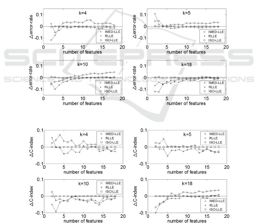
than zero except that the reduced dimension d is
among 14 to 18. For k=4, k=5, k=10 and k=18, the
∆error-rates of ISO-LLE are all close to zero. It can
be seen that the proposed RLLE method can produce
the lowest error-rate in most cases for the MNIST
dataset.
Figure 2 shows the change of the C-index
produced by RLLE, ISO-LLE and IED-LLE
compared to the C-index produced by LLE for the
MNIST dataset. In Figure 2, ∆C-index denotes the C-
index of RLLE, ISO-LLE or IED-LLE minus the C-
index of LLE. Similar to the ∆error-rate, when the
∆C-index produced by a method is less than zero, it
means that the method produces better results than the
LLE method. It can be seen from Figure 2 that when
k=4 the ∆C-indices produced by RLLE are all less
than zero except when d is 2, 10 or 12, and the ∆C-
indices produced by IED-LLE are all larger than zero
except d is within 14 to 18. When k=5 and k=10, the
∆C-indices produced by RLLE are all less than zero
except a special case (k=5, d=2), and the ∆C-indices
of IED-LLE are all less than zero except the cases:
(k=5, d=2 to 12), (k=10, d=2). When k=18, the ∆C-
indices of RLLE are all less than zero except that d is
within 16 to 18, and the ∆C-indices of IED-LLE are
all larger than zero except that d is within 2 to 5. For
k=4, k=5, k=10 and k
=18, the ∆C-indices of ISO-LLE
are also close to zero. So evaluated by the C- index,
RLLE can also produce better results compared to
LLE, ISO-LLE and IED-LLE on MNIST dataset.
Figure 3 shows the change of the error-rate
produced by RLLE, ISO-LLE and IED-LLE
compared to the error-rate produced by LLE for the
USPS dataset when k=4, k=8, k=10 and k=18. It can
be seen that for different values of k the ∆error-rates
produced by RLLE and IED-LLE are all less than
zero except a special case: (k=4, d=3). So for most
cases, the RLLE method can produce better results
Figure 1: ∆error-rate for the MNIST dataset.
Figure 2: ∆C-index for the MNIST dataset.
ICPRAM 2016 - International Conference on Pattern Recognition Applications and Methods
166
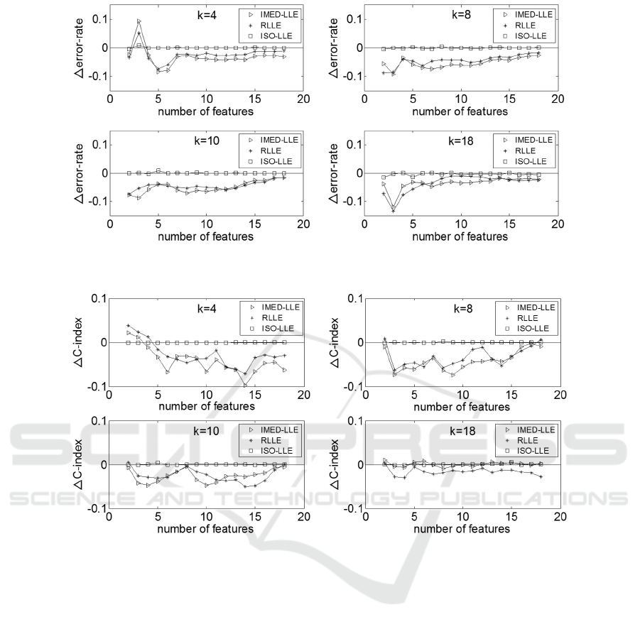
Figure 3: ∆error-rate for the USPS dataset.
Figure 4: ∆C-index for the USPS dataset.
than LLE. It is also noted that most of the ∆error-rates
produced by RLLE are larger than that produced by
the IED-LLE method. For k=4, k=8, k=10 and k=18,
the ∆error-rates of ISO-LLE are all close to zero. It
can be seen that the RLLE method can produce
smaller error-rates than LLE and ISO-LLE, but the
error-rates produced by RLLE are larger than IED-
LLE.
Figure 4 shows the change of the C-index
produced by RLLE, ISO-LLE and IED-LLE
compared to the C-index produced by LLE for the
USPS dataset. It can be seen in Figure 4 that when
k=4 the ∆C-indices of RLLE and IED-LLE are all less
than zero except that d is within 2 to 3. When k=8,
k=10 and k=18, the ∆C-indices produced by RLLE
are all less than zero except in some special cases
when the reduced dimension d is 2 or 18. When k=8
and k=10, the ∆C-indices produced by IED-LLE are
all less than zero. When k=18, the ∆C-indices of IED-
LLE are all close to zero. The ∆C-indices produced
by RLLE are larger than IED-LLE in most cases
when k=4, k=8 and k=10, and the ∆C-indices
produced by RLLE are all less than the IED-LLE
method when k=18. For k=4, k=8, k=10 and k=18, the
∆C-indices of ISO-LLE are all close to zero. It can be
seen that for most cases RLLE method can produce
better C-indices than LLE and ISO-LLE, and IED-
LLE can produce better C-indices than RLLE, which
is consistent with the results measured using error-
rate.
4.5 Discussion
In summary, for the MNIST dataset, the RLLE
method can produce the best results than LLE, ISO-
LLE and IED-LLE. For the USPS dataset, RLLE can
still produce better results than LLE and ISO-LLE in
Locally Linear Embedding based on Rank-order Distance
167

most cases. Although IED-LLE can produce better
results than RLLE when k=4, k=8 and k=10, the
results of RLLE are usually better than these of IED-
LLE when k=18.
It can be seen from Table 1 to Table 2 and from
Figure 1 to Figure 4 that if a distance measure can
find good nearest neighbor candidates, it can also
produce good dimension reduction results combined
with the LLE method. It can also be seen from the
experimental results that using C-index can produce
consistent evaluation results as using the error-rate.
One of the benefits of using C-index is that no
clustering process is needed after the dimension
reduction, which may avoid the bias of the selected
clustering algorithm in the evaluation of the
dimension reduction results.
5 CONCLUSIONS
In this work, we use the Rank-order distance instead
of the traditional Euclidean distance to find the
nearest neighbors and then produce low-dimensional
representation using a similar process as in LLE. It is
shown that the proposed RLLE method can realize
dimension reduction more effectively on the two
image datasets compared to LLE and ISO-LLE, while
producing competitive results compared to IED-LLE.
It is also shown that the Rank-order distance can find
better neighbors than the Euclidean distance and the
geodesic distance for representing local
configurations of the manifolds. The experimental
results also show that C-index is another good
indicator for evaluating the dimension reduction
results. Our future work will focus on reducing the
time complexity in the computation of the Rank-order
distance.
ACKNOWLEDGEMENT
This work is supported by the National Natural
Science Foundation of China (Grants No. 61272213).
REFERENCES
Belkin, M. & Niyogi, P., (2003) Laplacian eigenmaps for
dimensionality reduction and data representation,
Neural computation, 15 (6), 1373-1396.
Comon, P., (1992). Independent component analysis,
Higher-Order Statistics, 29-38.
Ding, C., He, X, & Zha, H. et al., (2002). Adaptive
dimension reduction for clustering high dimensional
data. Proceeding of the 2002 IEEE International
Conference on Data Mining, pp. 147-154.
Fukunaga, K., (1990). Introduction to statistical pattern
recognition, Academic press.
He, L.M., Jin, W. & Yang, X.B. et al., (2013). An algorithm
research of supervised LLE based on mahalanobis
distance and extreme learning machine. In: Consumer
Electronics, Communications and Networks (CECNet),
2013 3rd International Conference on. IEEE, pp. 76-
79.
Hinton, G. E. & Roweis, S.T., (2002). Stochastic neighbor
embedding. In: Advances in neural information
processing systems. pp. 833-840.
Hubert, L. & Schultz, J., (1976). Quadratic assignment as a
general data analysis strategy, British Journal of
Mathematical and Statistical Psychology, 29 (2), 190-
241.
Hull, J. J., (1994). A database for handwritten text
recognition research, IEEE Transactions on Pattern
Analysis and Machine Intelligence, 16 (5), 550-554.
Kouropteva, O., Okun, O. & Pietikäinen, M., (2002).
Selection of the optimal parameter value for the locally
linear embedding algorithm, Proc. 1st Int. Conf. Fuzzy
Syst. Knowl. Discov., pp. 359 -363.
LeCun, Y., Bottou, L. & Bengio, Y. et al., (1998) Gradient-
based learning applied to document recognition.
Proceedings of the IEEE, 86 (11), 2278-2324.
Pan, Y. & Ge, S.S., (2009). A. Al Mamun, Weighted locally
linear embedding for dimension reduction, Pattern
Recognition, 42 (5), 798-811.
Roweis, S.T. & Saul, L.K., (2000) Nonlinear
dimensionality reduction by locally linear embedding,
Science, 290 (5500), 2323-2326.
Saul, L.K. & Roweis, S.T., (2003). Think globally, fit
locally: unsupervised learning of low dimensional
manifolds, The Journal of Machine Learning Research,
4, 119-155.
Tenenbaum, B. et al., (2000). A global geometric
framework for nonlinear dimensionality reduction,
Science, 290 (5500), 2319-2323.
van der Maaten, J.P.L., Postma, E.O. & van den Herik, H.J.,
(2009). Dimensionality reduction: A comparative
review, Tilburg Univ., Tilburg, The Netherlands, Tech.
Rep. TiCC-TR 2009-005.
Varini, C. A., (2006). Degenhard, T.W. Nattkemper,
ISOLLE: LLE with geodesic distance,
Neurocomputing, 69 (13), 1768-1771.
Wold, S., Esbensen, K. & Geladi, P., (1987). Principal
component analysis, Chemometrics and intelligent
laboratory systems, 2 (1), 37-52.
Zhang, L. & Wang, N., (2007). Locally linear embedding
based on image Euclidean distance. In: Automation and
Logistics, 2007 IEEE International Conference on.
IEEE, pp. 1914-1918.
Zhang, X.F. & Huang, S.B., (2012). Mahalanobis Distance
Measurement Based Locally Linear Embedding
Algorithm, Pattern Recognition and Artificial
Intelligence, 25, pp. 318-324.
Zhang, Z. & Wang, J., (2006). MLLE: Modified locally
linear embedding using multiple weights. In: Advances
ICPRAM 2016 - International Conference on Pattern Recognition Applications and Methods
168

in Neural Information Processing Systems, pp. 1593-
1600.
Zhang, Z. & Zha, H., (2004). Principal manifolds and
nonlinear dimensionality reduction via tangent space
alignment, Journal of Shanghai University (English
Edition), 8 (4), 406-424.
Zhu, C., Wen, F. & Sun, J., (2011). A rank-order distance
based clustering algorithm for face tagging. In:
Computer Vision and Pattern Recognition (CVPR),
2011 IEEE Conference on. IEEE, pp. 481-488.
Zhuo, L., Cheng, B. & Zhang, J., (2014). A Comparative
study of dimensionality reduction methods for large-
scale image retrieval, Neurocomputing, 141, 202-210.
Locally Linear Embedding based on Rank-order Distance
169
