An Algorith to Derive Transfer Function Coefficients for an Auditory
Filterbank from Experimental Tuning Curves
Thomas Ostermann
Chair of Research Methodology and Statistics in Psychology, Witten/Herdecke University, 58313 Herdecke, Germany
Keywords: Cochlea, Filterbank, Lowpass, Transfer Function.
Abstract: Auditory processing is one of the most complex and fundamental tasks in human psychophysiology. In the
past 150 years researchers have tried to understand how sound and especially speech is processed in the human
ear. Today, digital auditory filter models and nonlinear active silicon cochlea models are used to simulate
cochlear sound processing. This article therefore aims at describing a simple algorithm to derive transfer
functions coefficients for an auditory filterbank from tuning curves. Based on the model of the basilar
membrane as a cascade of second order lowpass filters, the transfer functions are adopted to experimental
data of tuning curves in the cochlea. With basic information on the shape of the travelling waves the presented
algorithm is able to derive transfer function coefficients for an auditory filterbank. After the algorithm is
explained this article shows how to use it in the presence of experimental data, and gives an application to a
an operational amplifier filter circuit using active compensation.
1 INTRODUCTION
Auditory processing is one of the most complex and
fundamental tasks in human psychophysiology. In
the past 150 years researchers have tried to
understand how sound and especially speech is
processed in the human ear. While Helmholtz in his
book “On the sensations of tone as a physiological
basis for the theory of music” proposed a resonance
concept (Helmholtz, 1868), his idea was contradicted
by Wien (Wien, 1905), who stated that high
selectivity and high damping of the ear could
anatomically not be realized in the cochlea. On the
experimental site, von Bekesy found that frequency-
to-place transformation in the cochlea was not caused
by resonance but by traveling waves on the basilar
membrane (von Zimmermann, 1993; Ostermann et
al., 2002). In a variety of experiments on animal ears
post mortem von Bekesy measured the displacement
of the basilare membrane in a prepared cochlea for
tonal stimuli and displayed them as a function of
frequency with the maximal displaced normalized as
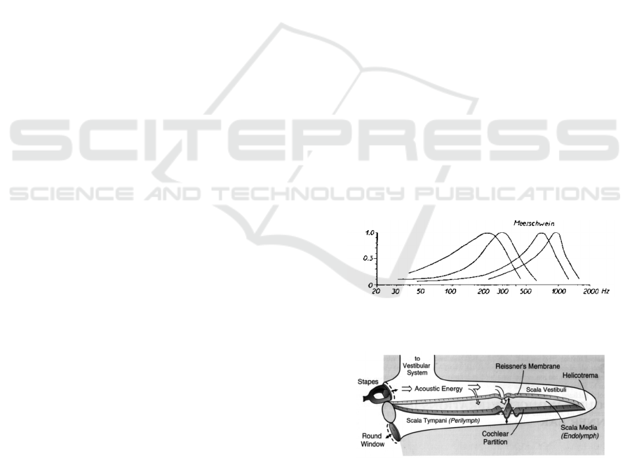
100% displacement (see Fig. 1 for an original graph
from Bekesy, 1944 and Fig. 2 for a schematic
drawing of the cochlea).
Mathematical modeling approaches like the
transmission-line models Peterson and Bogert
(Peterson and Bogert, 1950) or the hydrodynamical
model of Ranke (Ranke, 1950) very early proposed
the use of electronic filters for simulating cochlea
mechanics and finally led to the concept to model the
basilar membrane as a cascade of filters.
Figure 1: Normalized travelling waves on the basilare
membrane of the guinea pig (from Bekesy, 1944).
Figure 2: Schematic drawing and inner ear dynamics of the
Cochlea (from Wen, 2006).
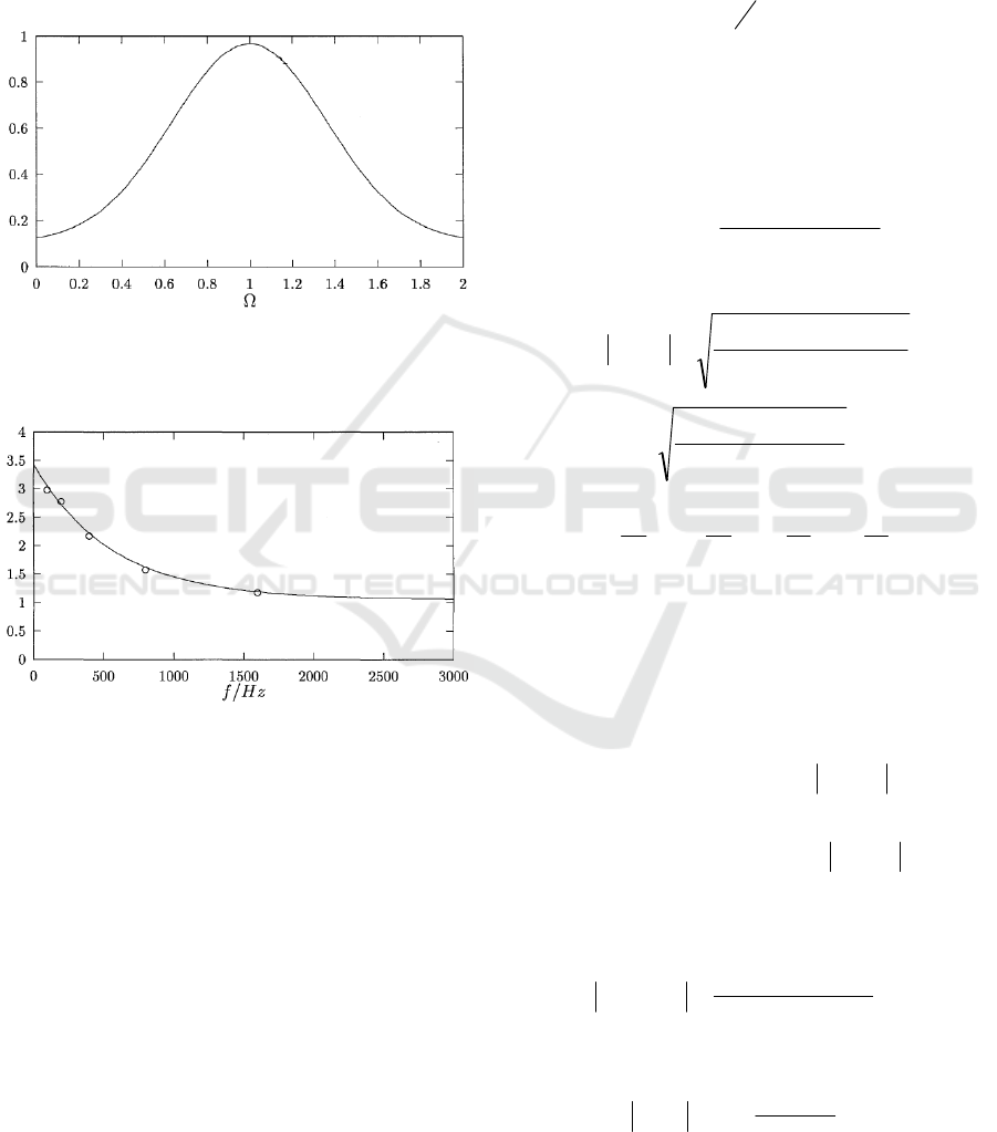
A non-logartithmic modeling approach for the
tuning curves is given in Fig. 3, while Fig. 4 gives
values for the renomalization of the travelling waves
in Fig 1.
194
Ostermann, T.
An Algorith to Derive Transfer Function Coefficients for an Auditory Filterbank from Experimental Tuning Curves.
DOI: 10.5220/0005657001940199
In Proceedings of the 9th International Joint Conference on Biomedical Engineering Systems and Technologies (BIOSTEC 2016) - Volume 5: HEALTHINF, pages 194-199
ISBN: 978-989-758-170-0
Copyright
c
 2016 by SCITEPRESS – Science and Technology Publications, Lda. All rights reserved

Several electronical models adopted the idea of a
filterbank to model the the cochlea. In 1972 David
presented a analogue lowpass filterbank of 64
cascaded 2
nd
order lowpass filters (David, 1972). A
similar model was constructed by Richter in 1977
which in addition contained electronical circuits to
simulate activen backcoupling in the basilare
membrane (Richter, 1977).
Figure 3: Modeling approach for a normalized tuning curve
h(Ω). Ω denotes the normalized frequency with respect to
f
max
(from Ostermann,1995).
Figure 4: Renomalization r(f) of the tuning curves (from
Ostermann,1995).
Today, digital auditory filter models have
replaced analogue filters and nonlinear active silicon
cochlea models are created using very large scale
integration (VLSI) to simulate cochlear sound
processing (Lyon et al., 2010; Katsiamis and
Drakakis, 2011). They are used in a variety of areas,
i.e. in the assessment of sound quality (Harlander et
al., 2014), for cochlea implants (Cosentino et al.,
2014), the recognition and analysis of speech emotion
recognition (Aher and Cheeran, 2014).
However the question still remains how to
determine the filter coefficients from the basis of
tuning curve data such as given in Fig 1.
This article describes therefore aim at describing
a simple and straightforward algorithm to derive
transfer functions coefficients for a auditory
filterbank from tuning curves.
2 MATERIAL AND METHODS
We first define f
max
as that frequency in which the
amplitude of the basilare membrane has its
maximum. Then
max
f
f
=Ω
denotes the normalized
frequency with respect to f
max
. Keeping in mind the
frequency-to-place transformation in the cochlea,
every frequency f is mapped to a unique place on the
basilare membrane.
Next the transfer function for a lowpass according
to (Furth and Andreou, 1995) is defined by
2
210
10
)(
Ω−Ω+
Ω+
=Ω
bibb
iaa
H
and its amplitude given by
()
22
1
2
2
20
22
1
2
0
)(
Ω+Ω−
Ω+
=Ω
bbb
aa
H
()
22
2
2
22
1
1
Ω+Ω−
Ω+
=
εγ
β
α
(1)
with
,
0
0
b
a
=
α ,
0
1
a
a
=
β ,
0
2
b
b
=
γ .
0
1
b
b
=
ε
Let h(Ω
N
) now denote the N
th
function of the
tuning curve given in figure 1 and r(f
gN
) denote the
renormalisation function for the peak of the tuning
curves (see figures 3 and 4), we can write the N
th
and
(N+1)
th
renormalized tuning curve as a product of
lowpass filters:
∏
=
Ω=Ω
N
i
igNN
Hfrh
1
)()()(
∏
+
=
++
Ω=Ω
1
1
11
)()()(
N
i
igNN
Hfrh
To obtain the transfer function of the (N+1)
th
lowpass
filter, we then get:
)()(
)()(
)(
11
1
gNN
gNN
N
frh
frh
H
Ω
Ω
=Ω
++
+
(2)
From Equation (1) we find that
)(
)(
)0(
1
gN
gN
fr
fr
H
+
== α
(3)
An Algorith to Derive Transfer Function Coefficients for an Auditory Filterbank from Experimental Tuning Curves
195

To ease the next calculations and without loss of
generality, α is set to 1 in the following calculations.
Next it is required that location and value of the
maximum of
)(
1+
Ω
N
H
correspond to the respective
values of
)()(
)()(
11
gNN
gNN
frh
frh
Ω
Ω
++
By calculating the first derivate
')(ΩH
, and equate
it to zero, we get
022
4422222
=Ω−Ω−−+ γβγεγβ
which leads to
2222
22
2
max
)(
11
εββγ
γββ
−++−=Ω
(4)
and it follows that
4
max
222
max
222
22 Ω−Ω−+= βγγβγε
(5)
Taking into account that
0
2
max
≥Ω
, equation (4) also
requires that
1)(
1
2222
≥−+ εββγ
γ
which is equivalent to
22
2 βεγ −≥
Inserting (5) into (1) leads to
22
22 22
max max max max
22
426
max max max max
()1 ()
() ()
HH
HH
ββ
γ
β
Ω−−Ω+Ω Ω
=
ΩΩ+ΩΩ
(6)
Finally |H(Ω)| for Ω=1 can be derived from the right
side of (2) and thus using (1) we have
()
2
2
2
1
1
)1(
εγ
β
+−
+
=H
which leads to
()
()
2
2
2
2
1)1( εγβ +−= H
(7)
By substituting and solving equations (5) to (7), the
remaining parameters can now be obtained. To
simplify the equations, we define the following
parameters:
)1(Ha = ,)(
max
Ω= Hb .
max
Ω=c
With
)(
)(
:)(
1
N
N
h
h
Ω
Ω
=ΩΨ
+
we finally get the algorithm
given in table 1:
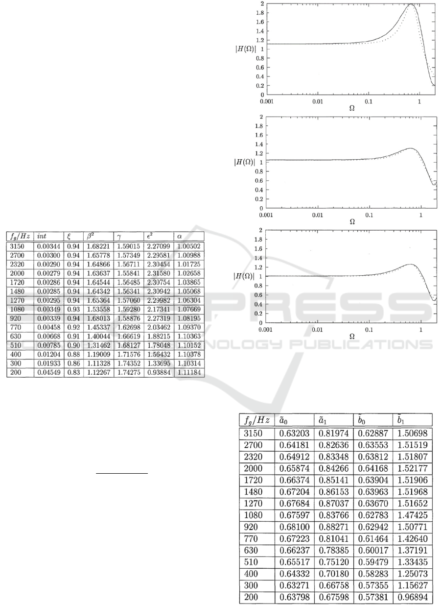
Table 1: Algorithm to determine the coefficients of the
transfer function.
For every N calculate:
)1(Ψ=a
)(
max1+
ΩΨ=
N
b
max1+
Ω=
N
c
422
422242222
2
)(
)221(
cba
cbcbcbcba
−
++−−−
=
β
26224
222222
)
1
bcbc
cbcb
β
ββ
γ
+
−−−
=
4222222
22 cc βγγβγε −−+=
3 RESULTS
The algorithm is now applied to experimental data.
Therefore the functions for h(
Ω ) and r(f) from Fig. 3
and Fig.4 have to be given explicitly. In (Ostermann,
1995) a nonlinear regression model was applied to the
experimental data and found the following equation:
))1(76.3exp(86.011.0)(
2
−Ω−⋅+=Ω h
(8)
and
)002.0exp(388.2052.1)(
gg
ffr ⋅−⋅+=
(9)
Using (8) we get
))(76.3exp(86.011.0
))1(76.3exp(86.011.0
)(
)(
2
1
2
11
1
2
2
1
gN
gN
gN
gN
f
f
N
f
f
N
N
N
h
h
++
−Ω−⋅+
−Ω−⋅+
=
Ω
Ω
+
++
A model fit with this algorithm for f
g
= 200Hz is
shown in Fig. 5.
Figure 5: Original curve (solid line) and model fit (dotted
line) for f
g
=200Hz.
HEALTHINF 2016 - 9th International Conference on Health Informatics
196

As can be seen the fitting quality is not sufficient
in the stopband region of the filter. Therefore, we
modified the algorithm given in table 1 with respect
to the parameter a:
),1(Ψ⋅= ξ a
with ξ ∈[0,1]
For every ξ the parameters ß
2
, γ and ε
2
are
calculated. In addition, the integral
[]
,)1(|)(|int
2
0
2
∫
ΩΨ−Ω= dH
which defines the area between the two curves in Fig.
5 is numerically minimized and that value of ξ is
chosen which minimizes the integral. Table 2
summarizes the results with respect to the cut-off
frequency f
g
:
Table 2: Parameters of int, ξ , β
2
. γ , ε
2
and α for cut-off
frequencies f
g
between 200 and 3150Hz.
To illustrate the results, Fig. 6 shows the original
curve and the model fit for the cut-off frequencies
200Hz, 1480Hz and 2700Hz.
The agreement of model fit and empirical data
increases with increasing cut off frequency. For a
transfer function H(s) with s=i
Ω
2
10
10
~~
~~
)(
ssbb
saa
sH
++
+
=
the coefficients
β
2
. γ , ε
2
and α given in Table 2
can easily be transformed. The respective values are
given in table 3.
Now, the coefficients for designing the filters are
given and can be applied to filter circuits using i.e.
operational amplifiers (OPAMS).
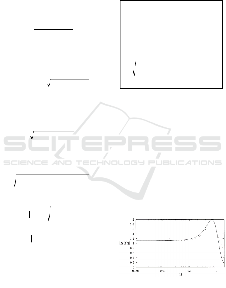
Figure 6: Original curve (solid line) and model fit (dotted
line) for f
g
=200Hz, 1480Hz and 2700Hz (top to down).
Table 3: Parameters of
1010
~~
,
~
,
~
bandbaa
for cut-off
frequencies f
g
between 200 and 3150Hz.
An Algorith to Derive Transfer Function Coefficients for an Auditory Filterbank from Experimental Tuning Curves
197

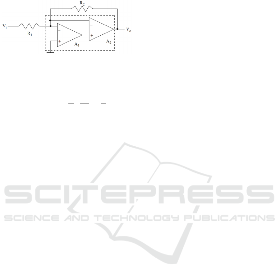
Figure 7: Example of a filter circuit using active
compensation from (Mohan, 2013).
The transfer function of this filter is given by
)1(1
1
)(
1
2
21
2
2
2
1
2
R
R
BB
s
B
s
B
s
R
R
sH
+++
+
−=
where R
1
and R
2
are the resistor values and B
1
and B
2
denote the unity gain bandwidths of the OPAMS.
4 CONCLUSIONS
Auditory filterbanks to simulate the cochlea have a
long history dating back to the 1950
th
. This article
presents an algorithm to derive transfer functions for
an auditory filterbank from experimental tuning
curves. Based on experimental data, tuning curves
were mathematically modelled and after some
transformations the coefficients of the transfer
function can be determined and be realized either in
analogue or digital filters.
Apart from the analysis of sound, such models can
also provide useful insights for students in the field of
auditory physiology i.e. to simulate patients’ hearing
loss. Such a system has actually been realized by
means of digital filters (Hohenberg et al., 2016).
This approach has also its limitations. It is based
on the assumption that tuning curves and frequency-
to-place transformation in the cochlea can be
modelled by a simple exponential approach. We also
assumed that the shape of the tuning curves does not
change. However, as Lyon et al., (2010) have pointed
out, physiological data show a filter shape
asymmetry. Finally this approach only models the
passive part of the cochlea. However there is also an
active back coupling which is not part of this
algorithm and has to be integrated by means of
positive feedback loop circuits (Ostermann, 2002;
Katsiamis et al., 2009; Elliott and Shera, 2012). Thus,
more extensive experimental analysis is needed to
validate the proposed algorithm.
However, if data can be modelled like in the
present article, this algorithm can be a part of a
straight forward approach to establish an auditory
filterbank.
ACKNOWLEDGEMENT
I would like to thank Roland Zieke, University of
Osnabrück, Germany for his support in this project.
REFERENCES
Aher, P., & Cheeran, A., 2014. Auditory Processing of
Speech Signals for Speech Emotion Recognition.
International Journal of Advanced Research in
Computer and Communication Engineering, 3(5),
6790-93.
Cosentino, S., Falk, T. H., McAlpine, D., & Marquardt, T.,
2014. Cochlear implant filterbank design and
optimization: A simulation study. IEEE/ACM
Transactions on Audio, Speech, and Language
Processing, 22(2), 347-353.
David, E., 1972. Elektronisches Analogmodell der
Verarbeitung akustischer Information in Organismen,
Habil.-Schrift, Universität Erlangen.
Elliott, S. J., Shera, C. A., 2012. The cochlea as a smart
structure. Smart Materials and Structures, 21(6),
064001.
Furth, P.M., Andreou, A.G., 1995. A Design Framework
for Low Power Analog Filter Banks. IEEE
Transactions on Circuits and Systems I: Fundamental
Theory and Applications, 42(11), 966-971.
Harlander, N., Huber, R., & Ewert, S. D., 2014. Sound
Quality Assessment Using Auditory Models. Journal of
the Audio Engineering Society, 62(5), 324-336.
Hohenberg, G., Reiss, G., Ostermann, T., 2016. An
interactive digital platform for teaching auditory
physiology using two classes of electronic basilare
membrane models. HEALTHINF 2016 - Proceedings of
the International Conference on Health Informatics.
Lyon, R. F., Katsiamis, A. G., Drakakis, E. M., 2010.
History and future of auditory filter models. In Circuits
and Systems (ISCAS), Proceedings of 2010 IEEE
International Symposium: 3809-3812.
Katsiamis, A., Drakakis E., Lyon R.F., 2009. A biomimetic,
4,5W, 120+dB, log-domain cochlea channel with ACG.
IEEE Journal of Solid-State Circuits, 44(3), 1006-1022.
Katsiamis, A., Drakakis E., 2011. Analogue CMOS cochlea
systems: A historic retrospective", Biomimetic Based
Applications, InTech, available from http://www.
intechopen.com/books/biomimetic based-applications/
analogue-cmos-cochlea-systems-a-historicretrospective,
2011.
Mohan, P. A., 2013. Active RC Filters Using Opamps. In
VLSI Analog Filters. Birkhäuser Boston: 13-146.
Ostermann, T., 1995. Parameterbestimmung zur
Modellierung der Schallwirkung in der Cochlea
mittels elektronischer Bauteile. Diplomarbeit im
Fachbereich Mathematik der University of Osnabrück.
HEALTHINF 2016 - 9th International Conference on Health Informatics
198

Ostermann, T., Zielke, R., David, E., 2002. Eine
mathematisch-technische Modellierung von passiven
und aktiven Schwingungsformen der Basilarmembran.
Biomedical Engineering, 47(1-2), 14-19.
Peterson, L., Bogert, B., 1950. A dynamical theory of the
cochlea. JASA 22, 369-381.
Ranke, O.F., 1950. Hydrodynamik der Schnecken-
flüssigkeit, Zs. f. Biol. 103, 409-434.
Richter, A.,1976. Ein Funktionsmodell zur Beschreibung
der amplitudenabhängigen selektiven Eigenschaften
des Gehörs. Dissertation, TU München.
Von Békésy, G., 1944. Über die mechanische
Frequenzanalyse in der Schnecke verschiedener Tiere.
Akust. Z., 9, 3-11.
Von Helmholtz, H. , 1865. Die Lehre von den Tonempfin-
dungen als physiologische Grundlage für die Theorie
der Musik. Vieweg, Braunschweig.
Wen, B., 2006. Modeling the nonlinear active cochlea.
Doctoral dissertation, University of Pennsylvania.
Wien, M., 1905. Ein Bedenken gegen die Helmholtzsche
Resonanztheorie des Hörens. In: Festschrift Adolph
Wüllner gewidmet zum 70. Geburtstage. Teubner,
Leipzig: 28–35.
Zimmermann, P., 1993. Entwicklungslinien der Hörtheorie.
NTM International Journal of History & Ethics of
Natural Sciences, Technology & Medicine, 1(1), 19-36.
An Algorith to Derive Transfer Function Coefficients for an Auditory Filterbank from Experimental Tuning Curves
199