
Decentralized Gradient-based Field Motion Estimation with a
Wireless Sensor Network
Daniel Fitzner and Monika Sester
Institute of Cartography and Geoinformatics, Leibniz University, Hannover, Germany
Keywords: Motion Estimation, Optical Flow, Wireless Sensor Network, Spatio-temporal Field.
Abstract: Information on the advection of a spatio-temporal field is an important input to forecasting or interpolation
algorithms. Examples include algorithms for precipitation interpolation or forecasting or the prediction of
the evolution of dynamic oceanographic features advected by ocean currents. In this paper, an algorithm for
the decentralized estimation of motion of a spatio-temporal field by the nodes of a stationary and
synchronized Wireless Sensor Network (WSN) is presented. The approach builds on the well-known
gradient-based optical flow method, which is extended to the specifics of WSNs and spatio-temporal fields,
such as spatial irregularity of the samples, the strong constraints on computation and communication and the
assumed motion constancy over sampling periods. A specification of the algorithm and a thorough
analytical analysis of its communicational and computational complexity is provided. The performance of
the algorithm is illustrated by simulations of a sensor network and a spatio-temporal moving field.
1 INTRODUCTION
Information on the advection of dynamic features in
the atmosphere or in the ocean is an important input
to estimation algorithms. Examples include
algorithms for precipitation field interpolation
(Fitzner and Sester, 2015), nowcasting (Bowler et
al., 2004) or the prediction of the evolution of
oceanographic features advected by ocean currents.
In this paper we investigate, how the advection of
spatio-temporal dynamic features, modelled as
spatio-temporal fields of a scalar attribute value, can
be estimated decentralized by the nodes of a
Wireless Sensor Network (WSN) deployed within -
and sensing the field.
For estimating the motion, a gradient-based
optical flow algorithm is used as a basis and adjusted
to the specifics of WSNs and spatio-temporal fields,
i.e. the irregularity of samples, the strong constraints
on communication and computation and the
assumed motion constancy over sampling periods
(see Section 4 for a more thorough elaboration on
the specifics of WSNs and spatio-temporal fields).
The main contributions of the work can be
summarized as follows:
- Approach for Estimation of Optical Flow
Gradient Constraints in the Network. We
provide an approach for the estimation of the
required partial derivatives (i.e. the gradient
constraint, see Section 3.2 on optical flow) of the
field from irregular sensor data as well as a
methodology for error estimation inspired by the
calculation of error measures from satellite
configurations for GPS positioning.
-
Incremental Field Motion Estimation. A kalman
filter based formalization of the optical flow
equations is provided, in order to account for
motion vector correlation over sampling steps
and to allow efficient real-time processing in the
network by each node.
-
Decentralized Algorithm Specification and
Complexity Analysis. A decentralized pseudo-
code specification of the algorithm is provided,
using the structure and formalisms provided by
(Duckham, 2012), as well as a thorough analysis
of its communication and computational
complexity.
The proposed algorithm requires the specification of
only three parameters with clear-cut interpretations:
the maximum communication distance in between
the sensor nodes, which is, in a real deployment of a
WSN, determined by the physical hardware. Further
parameters are the kalman filter prediction and
measurement noise covariances.
The paper is structured as follows. In Section 2,
Fitzner, D. and Sester, M.
Decentralized Gradient-based Field Motion Estimation with a Wireless Sensor Network.
DOI: 10.5220/0005639100130024
In Proceedings of the 5th International Confererence on Sensor Networks (SENSORNETS 2016), pages 13-24
ISBN: 978-989-758-169-4
Copyright
c
2016 by SCITEPRESS – Science and Technology Publications, Lda. All rights reserved
13

the relevant related work is introduced, mainly those
concerned with the estimation of properties of
spatio-temporal fields, such as peaks, pits or
boundaries. In Section 3, the employed WSN and
field model as well as the basics of image-based
optical flow are provided. Section 4 contains the
theory of the proposed approach and Section 5 the
algorithm specification. In Section 6, the
performance of the algorithm is illustrated by means
of a simulated dynamic field and sensor network.
Section 7 discusses possible extensions of the
proposed method and concludes.
2 RELATED WORK
There exists a significant body of work on the
estimation of properties of dynamic spatio-temporal
fields with WSN. Problems include the estimation of
field boundaries (Sester, 2009), identification of
critical point such as peaks and pits (Jeong et al.,
2014) or even spatial interpolation in the network
(Umer et al., 2010). The book of (Duckham, 2012)
provides a thorough overview on this topic as well
as a description of the advantages of decentralized
computation in the network, which also apply to the
work presented in this paper.
Another research line related to our work is the
tracking (here, in the meaning of following) of
advected spatio-temporal features by mobile nodes
(Brink and Pebesma, 2014), (Das et al., 2012).
While in these works mobile nodes are assumed that
can either move by themselves (Brink and Pebesma,
2014) or are advected with the field, e.g. buoys
advected by ocean currents (Das et al., 2012), our
work assumes a network of stationary sensors and
aims at estimating the motion from the time series of
sensor measurements.
Further, there is a significant amount of work on
object tracking with WSNs, i.e. generating
information on the trajectory of a mobile object
without necessarily following it, such as (Tsai et al.,
2007). However, to the best of our knowledge, the
problem of estimating field (not object-) motion of a
spatio-temporal field within a network of stationary
sensor nodes has not been tackled so far.
3 BACKGROUND
3.1 Network and Field Model
Throughout the paper, a sensor network is modelled
as a graph , where is the set of sensor
nodes distributed on the plane and is the set of
communication links between nodes. The allowed
bidirectional communication links are solely
determined by a maximum Euclidean
communication distance r in the plane and hence,
is a unit disk graph (UDG). We assume that a node
∈ knows its position
,
on the plane,
e.g. by GPS. Further, the nodes are able to sense a
real-valued scalar spatio-temporal field
:
→ where ,,
is a location in the
space-time cube (and
indicates matrix
transposition). A particular sensor measurement of
sensor
at timestep is denoted with
,
where
,
,
,
.
3.2 Gradient-based Motion Estimation
Optical flow methods such as (Lucas et al., 1981) or
(Horn and Schunck, 1981) are usually employed for
estimating pixel displacement (motion) in between
two images and use image derivatives for
estimation. They have successfully been applied for
computing the motion of spatio-temporal fields, e.g.
from weather radar images (see e.g. (Bowler et al.,
2004) or (Fitzner and Sester, 2015), mainly for
nowcasting purposes. The underlying assumption of
optical flow is that the intensity (pixel / field values)
remains constant in between the sampling periods
and a change in values for a particular location
solely comes from field motion. Formally, this
means that there exists a vector in the space-time
cube ∆,∆,∆
such that Equation (1) holds.
(1)
Gradient-based optical flow methods are further
based on the assumption that a first-order taylor
series expansion of the field values is adequate, as
displayed in Equation (2).
≅
∆
∆
∆
(2)
where
,
and
are the partial derivatives in
space and time directions resp. Equation (2) is called
the linearity assumption of optical flow, as higher
order terms are ignored. Combining (1) and (2) and
dividing by ∆ then results in the gradient constraint
equation of (3).
∆ ∆
⁄
∆ ∆
⁄
≅0
(3)
Instantiating the gradient constraint equation (3)
requires estimates of
,
and
. Usually, they
are estimated with numerical differentiation using
neighboring (in space and time) pixel values.
Estimating motion
∆ ∆
⁄
and
∆ ∆
⁄
SENSORNETS 2016 - 5th International Conference on Sensor Networks
14

then requires at least two gradient constraints to be
integrated. More than two constraints are usually
integrated over a pixel neighborhood by least
squares adjustment (Lucas et al., 1981), (Fleet and
Weiss, 2006).
4 MOTION ESTIMATION WITH
A WSN
Estimating spatio-temporal field motion from
irregular sensor data differs from image based
optical flow, in that:
1. The data is irregular, i.e. the samples are not
aligned along the coordinate axes and direct
estimation of the partial derivatives, e.g. via
forward-, backward-, or even central numerical
differentiation, as e.g. proposed by (Horn and
Schunck, 1981) is not possible. The methodology
for estimating the required partial derivatives
from irregular data is described in Sections 4.1
and 4.2.
2. For estimating field motion with a WSN, it is
likely that the motion per sampling timestep is
smaller than the spacing in between sensor nodes
(this corresponds to subpixel motion in images).
For example, considering two sensors with a
sampling interval of 1-minute, a spacing of 1 km
in between and a spatio-temporal field moving
with a velocity of 60 km/h. In this case, the
spacing is equal to the field motion per sampling
time step. However, for the use cases imagined,
we consider 60 km/h as being already rather fast
and 1 km spacing as rather dense. For example,
the average density of rain gauges in Germany is
one station per 1800 km² (Haberlandt and Sester,
2010). Therefore, in the remainder of this paper.
it is assumed that the motion is small compared
to sensor spacing. For such cases of “subpixel”
motion, a gradient-based method is adequate, as
e.g. described by (Huang and Hsu, 1981). This
assumption of small motion is directly
implemented in the weighting scheme for the
estimation of partial from directional derivatives,
described in Section 4.4.
3. In contrast to image-based optical flow, it is
likely that the motion is correlated over several
sampling periods. For example, (Zawadzki,
1973) concludes that the taylor hypothesis on
frozen turbulence, which is closely related to the
optical flow assumption of (1), is valid for
precipitation for time periods shorter than 40
minutes. Therefore, it is likely that past field
motion can be used to improve the estimate of
current field motion. A kalman filter
formalization of this assumption is presented in
4.5.
4. Finally, in contrast to motion in images, a-priori
knowledge on the motion properties can be
assumed. For example, wind speed statistics exist
or information on the advection of rainclouds. In
a real-world application of the algorithm, this
domain knowledge can be used to specify the
required parameters, mainly concerning the
kalman prediction and measurement noise
covariances.
4.1 Estimating Directional Derivatives
When the data is irregularly sampled in space and
time, estimating the partial derivatives directly is
impossible, as there might be no samples aligned
along the coordinate axes. Therefore, the partial
derivatives need to be estimated from the directional
derivatives in the space-time cube, defined as
displayed in Equation (4).
´
lim
||→
||
(4)
where
,
,
is a separation vector in the
space-time cube, is a spatio-temporal location and
|
|
.
For any pair of sensor samples
,
and
,
of sensors
and
and timesteps and
(where is also allowed when and vice
versa), an estimate of the directional derivative of
Equation (4) can be calculated using forward
differentiation along the particular direction, as
displayed in equation (5).
̂
,
´
,
,
,
|
,
|
(5)
where
,
is the spatio-temporal distance vector
between the spatio-temporal locations
,
and
,
and
,
and
,
are field measurements at the
these locations.
4.2 Estimating the Gradient Constraint
Estimating the partial derivatives required for optical
flow using a set of estimates of directional
derivatives of the form of (5) requires some form of
adjustment, e.g. least squares adjustment, to be
performed by each sensor. The functional
relationship between the estimate of a particular
Decentralized Gradient-based Field Motion Estimation with a Wireless Sensor Network
15
directional derivative and the partial derivatives
along the space-time cube coordinate axes is
displayed in Equation (6). For easing readability, we
skip the spatio-temporal position
,
, indicating the
position of the particular sensor
at time .
̂
,
´̂
̂
̂
(6)
where
,
,
,
is the unit vector in the
particular spatio-temporal direction
,
, ̂
,
´ is
the directional derivative estimated with (5) and ̂
,
̂
and ̂
are the partial derivatives to be estimated.
A set of such linear equations available at a specific
spatio-temporal sensor position
,
then allows
calculating ̂
, ̂
and ̂
. In matrix form, the linear
system to be solved is:
(7)
where is the 3 matrix of unit vectors at
,
,
3 is the number of directional derivatives
available and ̂
,̂
,̂
is the 31 vector of
partial derivatives to be estimated.
is the 1
vector of known estimates of directional derivatives.
An approximate solution to the equation is given by
the least-squares estimator displayed in Equation (8).
argmin
(8)
where
‖
.
‖
is the
- or Euclidean norm. The
minimization is then performed by solving the
normal equations for the vector of partial derivatives
, as displayed in Equation (9).
(9)
The weight matrix contains a weight for each
estimate of a directional derivative. Certainly, the
weight should be a function of field properties and
the distance |
,
|. In Section 4.4., the methodology
for the estimation of weights is described.
4.3 Requirements on Node Stationarity
and Sampling Synchronicity
As the distance vector is a vector in space and
time, the calculation of the length
|
|
requires the a-
priori specification of a spatio-temporal anisotropy
factor such as a decision on the unit of measures. If
this knowledge is available a-priori, the sensors are
allowed to move and sample the field
asynchronously, i.e. at different time steps.
However, in this work, it is assumed that the
anisotropy factor is not known. Therefore, the
assumptions of node stationarity and time
synchronicity are essential. In this case, space can be
treated separated from time and there are always
neighboring sensor samples in space only and time
only available, while those in space-time can be
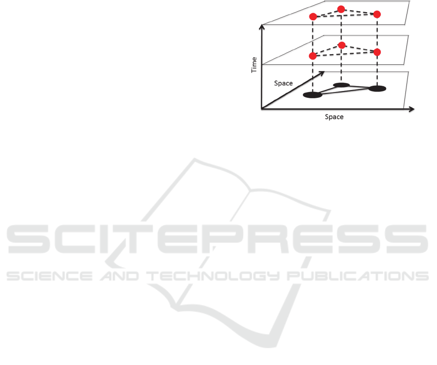
ignored. In Figure 1, a visualization of this
assumption is displayed.
Figure 1: Assumption of node stationarity and sampling
synchronicity. Red dots represent sensor measurements,
which are taken at fixed spatial sensor positions at
synchronized time steps / periods.
Another advantage is that the amount of
computation within and communication between the
nodes can be reduced, since the sensors need to
communicate their position only once, as it (and
hence matrix as well) is constant. Constancy of
depends on the chosen weight. In Section 4.4, a
weight is proposed that is solely derived from the
spatial configuration. Therefore, each sensor can
compute
once, reducing
computational and communication costs per
timestep. Further, the estimation of the temporal
derivative does not have to be part of the linear
system of (7). The temporal derivative can be
estimated by each sensor using simple backward
differencing along the time axis. Further, the
temporal difference between sampling steps can be
set to be equal to 1, i.e.
,
1. This way, the
estimated temporal derivative is equal to the
difference between current and previous value, i.e.
,
,
for a particular sensor
and no
division is required.
4.4 Derivative Weighting and Gradient
Constraint Error Estimation
From the assumptions described in 4.3 follows that
the partial derivative along the time axis can be
directly estimated. Therefore, no error for the
estimated temporal derivative is assumed. For
estimating the error (and therefore the weight)
associated with the estimate of a particular
directional derivative in space, the heuristic
SENSORNETS 2016 - 5th International Conference on Sensor Networks
16

displayed in Equation (10) is used:
(10)
where is the maximum possible communication
range between sensors,
is spatial distance
between the two sensors
and
. The weight
matrix then contains the inverse distance 1/
as
the weight.
The individual error associated with a gradient
constraint can then be estimated from individual
direction derivative errors using the law of
propagation of error (see e.g. (Langley, 1999) for an
application to GPS or any textbook on adjustment
theory adjustment for the derivation of the formula):
(11)
where
is the 22 covariance matrix of the 21
vector of estimated partial derivatives . The overall
quality of a gradient constraint is then computed as
the sum of the diagonal elements of
, similar to
the calculation of the positional error variance in
GPS positioning (Langley, 1999).
(12)
This way, a gradient constraint error variance
reflects the spatial neighborhood configuration of
the node
generating the constraint. Since field
properties have been ignored in Equation (10), the
value
is not a proper representation of a single
gradient constraint error but only a proper
representation of the error relationships between
gradient constraints. Therefore, when the error is to
be used in the motion estimation algorithm described
in the next section, it has to be transformed to the
proper level of error for the specific field under
consideration. The approach used here is to scale an-
priori known gradient constraint error variance by
. In the evaluations, it is shown that this, which
we call configuration-based error, indeed provided
improved motion estimates compared to a uniform
weighting and uniform error.
4.5 Kalman Filter for Incremental
Motion Estimation
Depending on sampling rate and field properties, the
motion vector at a particular position might be
considered constant or at least highly correlated in
between sampling periods. A particular model that
fits nicely to this problem of real-time incremental
estimation of a real-valued vector is the kalman filter
(Kalman, 1960). In the following, the theoretical
model of the kalman filter is described with a
specific focus on the problem of motion estimation.
The implementation then follows standard
implementations as described e.g. in (Greg Welch,
2006).
The kalman filter assumes a hidden state in the
form of a real-valued column-vector that can not
directly be measured, in our case, the field motion at
a particular time step , displayed in (13).
,
,
,
(13)
where
,
and
,
are the motion vector
components in direction and , resp. (again,
subscripts concerning sensor node are omitted as
each node is assumed to implement the filter).
The error of the state is formalized in an error
covariance 22matrix
. The filter then assumes
that a current state is a linear function of a past state
plus some mean-zero Gaussian noise with a
certain covariance , i.e. ~0, Q), as displayed
in Equation (14).
(14)
where is the matrix that transforms past to current
state and hence describes motion evolution at the
particular sensor position. To keep the model and
computations simple, motion constancy in between
sampling periods is assumed and therefore, is the
identity matrix. In addition to motion evolution, the
kalman measurement model describes, how noisy
measurements are related to the state:
(15)
where
is the measurement,
is the linear
function that maps
to the measurement and
~0, is zero-mean Gaussian noise with
covariance . In order to use (15) for updating the
motion state with a new gradient constraint instance,
the constraint of (3) has to be recast into the linear
regression form (see Särkkä (2013) or Watson
(1983) for the theory on kalman filtering for linear
regression problems). Then, the temporal derivative
is considered a linear function of the motion
components:
,
,
(16)
Here,
is considered the measurement, i.e.
,
,
is the measurement matrix
and
,
and
,
is as above. This way, the motion
state is updated with new gradient constraints. Since
is scalar, is scalar as well and therefore, solving
the kalman update equations does not require matrix
inversion (Särkkä, 2013), which is advantageous for
Decentralized Gradient-based Field Motion Estimation with a Wireless Sensor Network
17

the amount of processing required. Essential is the
specification of an a-priori state, which can only be
set to the zero vector. The a-priori uncertainty
should contain large values on the diagonal,
indicating the low confidence in the initial state. The
uncertainty associated with prediction., depends on
the temporal sampling rate, i.e. the time difference
between kalman filter steps, as well as the assumed
motion constancy of the spatio-temporal field. The
scalar measurement noise variance is a direct
function of gradient constraint accuracy. In this
work, it is derived from the accuracies of the
directional derivatives, as described in Section 4.4.
Further, it depends on the spatial distance between
the sensor estimating the motion and the sensor
estimating the gradient constraint. The assumption
is: the closer the two sensors are the more similar is
the motion.
In addition, as described in work on image-based
optical flow such as (Lucas et al., 1981), the gradient
constraint accuracy depends on field properties at
the site where the gradient constraint is constructed.
Including these properties (spatial distance and field)
into the approach is subject to future extensions of
the algorithm, which are further discussed in Section
7.
5 ALGORITHM PROTOCOL
For specifying the algorithm, the protocol structure
and pseudo-code elements of (Duckham, 2012) are
used.
Protocol: Field Motion Estimation
Restrictions: Graph , with nodes
∈ with
constant positions and comm. links . Function : →
returning neighbours of a node.
:→ returning
neighbours with >1 neighbours.
Initialization: All nodes in state INIT
Data: Each node
∈ implements the kalman filter (Section
4.5) and stores matrix and the errors associated with the
gradient constraints provided by itself or neighbors.
Parameters: Max. communication range , kalman parameters
and .
INIT
broadcast (
,
)
if
|
|
< 2
become PROCESSING
Receiving other node position
,
if
|
|
> 1
compute |
|
compute unit vector
Add
to
Add 1/
to
if
|
|
|
|
compute
compute
broadcast
to
become PROCESSING
PROCESSING
(1) Whenever new sample
,
is available
broadcast ,
,
if
|
|
> 1
compute kalman prediction step
compute temporal derivative
̂
´
,
,
(2) Receiving sample ,
,
from neighb.
if
|
|
> 1
compute ̂
´
Add ̂
´ to
if
|
|
compute
compute kalman update with
broadcast to
(3) Receiving gradient constraint (,)
if
|
|
> 1
compute kalman update with
In the INIT step, a sensor distributes its position to
all neighbors. If it has only zero or only a single
neighbor, it is not able to estimate partial derivatives
and hence, proceeds to state PROCESSING.
Otherwise, it waits for receiving the positions of all
neighbors. If it has done so, the matrix can be
computed, the error
associated with the node can
be broadcast and the node is ready for motion
estimation (i.e. state PROCESSING).
At each new sampling step (1) of a sensor, a
kalman prediction on the motion is performed and
the temporal derivative is calculated. Further, the
sensor measurement is transmitted to the neighbors.
When a new sample from a neighboring sensor
arrives (2), the current directional derivative is
estimated and added to the derivative vector
. If
is filled with all data from participating neighbors,
the gradient constraint is computed, which is then
used for kalman update and transmitted to all
neighbors participating in motion estimation. When
a gradient constraint from a neighboring sensor
arrives (3), the kalman update step is executed as
well.
5.1 Algorithm Analysis
For analyzing the complexity of the proposed
algorithm, we follow the approach of (Duckham,
2012) and focus on the overall amount of
communication required (Section 5.1.1). Further, the
amount of computation performed by each node is
analyzed in Sections (5.1.2) and (5.1.3). For doing
this, the widely used notion of a flop is employed,
representing a floating point operation such as
addition, multiplication or division (see e.g. (Golub
SENSORNETS 2016 - 5th International Conference on Sensor Networks
18

and Loan, 1996) for an introduction to flops and
their usage in analyzing matrix computations).
5.1.1 Communication Complexity
In terms of communication complexity, the
algorithm requires an initial broadcast of the sensor
positions and the error associated with the gradient
constraints provided by a sensor. Therefore,
|
|
|
|
messages are sent at the INIT state, where
is the whole set of sensor nodes and
⊆ is the
subset of sensor nodes with at least 2 neighboring
nodes. Then, each timestep, each sensor sends the
sensed value and each sensor with at least 2
neighboring nodes sends the estimated partial
derivatives in addition, i.e. the gradient constraint.
Therefore, the number of sent messages per timestep
is
|
|
|
|
.
5.1.2 Complexity of Derivative Estimation
Estimating the partial derivative along the temporal
axis requires a single subtraction of values and no
multiplications / divisions at each timestep.
Estimating the partial derivatives in space from
neighboring sensor measurements requires the
computation of
once at the
INIT state of the algorithm, plus multiplication
with the vector of the estimates of directional spatial
derivatives at each timestep.
Processing Costs at INIT Step:
Building the Matrices: The computation of a
directional derivative requires computing the
Euclidean distance to each neighboring node. This
requires 2 subtractions, 2 multiplications and a
square root. Building the unit vectors then requires
another 2 divisions. In addition, building the weight
matrix requires divisions. Hence, in total
6 flop plus a square root are required. For
example, a sensor with 5 neighbors requires 35 flop
and a square root computation for building the
required matrices and vectors
Computing
: is a 2
matrix, where is the number of neighboring
sensors. is a diagonal matrix of weights.
Therefore, due to being diagonal, matrix
multiplication
requires 2 multiplications
and no additions and results in a 2 matrix.
Subsequent multiplication with requires additional
22 multiplications and 221
additions. Inverting the resulting 22 matrix
requires 2 multiplications and one
subtraction for the determinant plus 4 divisions.
Multiplication with the already computed
then
requires 22 multiplications and 2
additions and results in the 2 matrix to be
available for partial derivative estimation at each
timestep. Computing the gradient constraint error
from the already computed
requires a
single addition, as shown in Equation (12). For
example, a sensor with 5 neighbors requires 84 flop
for computing and
.
Processing Costs at PROCESSING Step:
At each timestep, the resulting 2 matrix is to
be multiplied with directional derivative 1
vector
, requiring 2 multiplications and 2
1 additions. For example, a sensor with 5
neighbors requires 18 flop per timestep for
estimating the required partial derivatives in space.
5.1.3 Complexity of Motion Estimation
The computations in the kalman prediction and
update steps are independent from the number of
neighbors . However, while the prediction step is
executed once per timestep, the update step is
executed times per timestep.
Prediction Step: The kalman prediction step
requires a single matrix addition of the two 22
matrices and . As is diagonal, this requires
two additions or 2 flop.
Update Step: The following analyses rely on a
standard kalman filter implementation with the
matrices as described in Section 4.5. The main part
is the computation of the kalman gain matrix.
Computing
requires 4 multiplications and 2
additions. Subsequent multiplication with
requires 2 multiplications and a single addition and
results in a scalar value to be added to measurement
error variance . The resulting value is inverted,
requiring a single division. Multiplying with the
already computed
requires 2 multiplications
and results in the 21 kalman gain matrix . In
total, 13 flop are required for kalman gain
computation. Updating with a new measurement
requires 2 multiplications and one addition for
, a subtraction and the subsequent scalar
multiplication with the kalman gain vector. The
resulting vector is added to the state, requiring two
additions. In total, 8 flop are required for updating
the state with a new measurement. Updating the
error covariance matrix requires 4 multiplications, 4
subtractions for
plus another 8
multiplications and 4 additions for the multiplication
with the previous error covariance matrix
. In
total, 20 flop are required for updating
to
.
Decentralized Gradient-based Field Motion Estimation with a Wireless Sensor Network
19
Therefore, the motion estimation update step
requires 41 flop per neighbour per timestep.
6 EMPIRICAL EVALUATION
6.1 Evaluation Methodology
6.1.1 Simulation of Moving Field and Sensor
Network
For evaluation, a set of 25 sensor nodes is
distributed on the unit square, with a maximum
communication range of 0.25. In addition, a
gaussian field of the form of (17) is simulated on a
larger square.
,
,
,
∗
(17)
where is the number of gaussians,
,
is the x-
coordinate,
,
is the y-coordinate of the center of
gaussian and
is the variance. Due to the
linearity assumption of optical flow of Equation (2)
and (3), it is clear that the motion estimation works
well, when the field is approximately linear at the
sites where the gradient constraints are constructed.
The degree of linearity of the simulated field can be
controlled by the parameters and
: the larger the
number of gaussians and the smaller
, the less
linear is the simulated field. Therefore, for
evaluation, the field is computed from a large
number of 300 gaussians using Equation (17),
each with a variance randomly chosen from the
small interval [0, 0.01] and a center position
,
,
,
randomly chosen on the larger square.
The simulations are executed over 50 timesteps
and each of the 25 nodes samples the field at each
timestep. Further, at each timestep, the whole field is
displaced along a particular motion vector, i.e. the
variances of the gaussians remain constant while the
center coordinates (
,
,
,
) are shifted uniformly.
In some of the experiments presented below, the
motion vector is also manipulated at each timestep
with a constant acceleration in both directions.
Further, in some experiments, the motion is spatially
inhomogeneous, which means each gaussian moves
differently depending on its current location in the
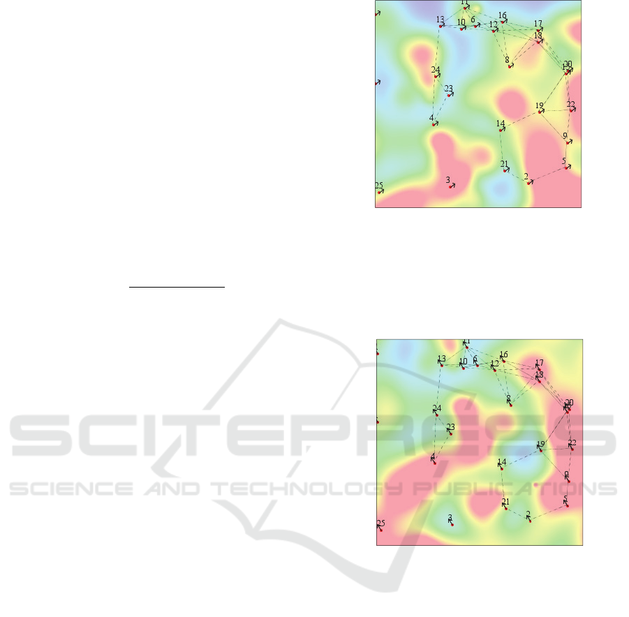
unit square. In Figure 2, a snapshot of the field, the
sensor network with node ids and true motion
vectors (per timestep) is displayed.
Figure 2: Snapshot of the simulated field, sensor network
and true motion vectors at the beginning of a simulation
run.
Figure 3 displays the situation 20 timesteps later,
with a displaced field and the current (changed) true
motion vector.
Figure 3: Snapshot of the simulated field, sensor network
and true motion vectors, 20 timesteps after the snapshot of
Figure 2.
6.1.2 Kalman Filter Initialization and
Parameters
The filter for motion estimation implemented by
each node is initialized with an initial motion state
estimate of
0,0
and an initial error
covariance matrix
containing arbitrarily chosen
large values on the diagonal, indicating the low
confidence in the initial motion state. The remaining
parameters and have been specified based on
visual evaluations of the motion estimation results. It
has turned out that the motion estimation
performance increased with significantly lower
assumed error for the prediction than for
measurement. This can be explained by the rather
low accuracy of the individual gradient constraints.
SENSORNETS 2016 - 5th International Conference on Sensor Networks
20
6.2 Results
In the following, some results of the generated
motion information are provided in order to explain
the performance of the proposed algorithm. In the
first experiment of Section 6.2.1, constant motion in
space and time is simulated. Then, in Section 6.2.2,
a spatially varying motion field is generated, that is
constant in time. In another experiment described in
Section 6.2.3, the motion vectors are manipulated by
a constant acceleration. Finally, in Section 6.2.4, it is
shown that a configuration-based kalman
measurement error indeed provides an improvement
compared to a fixed error that is independent of the
spatial configuration.
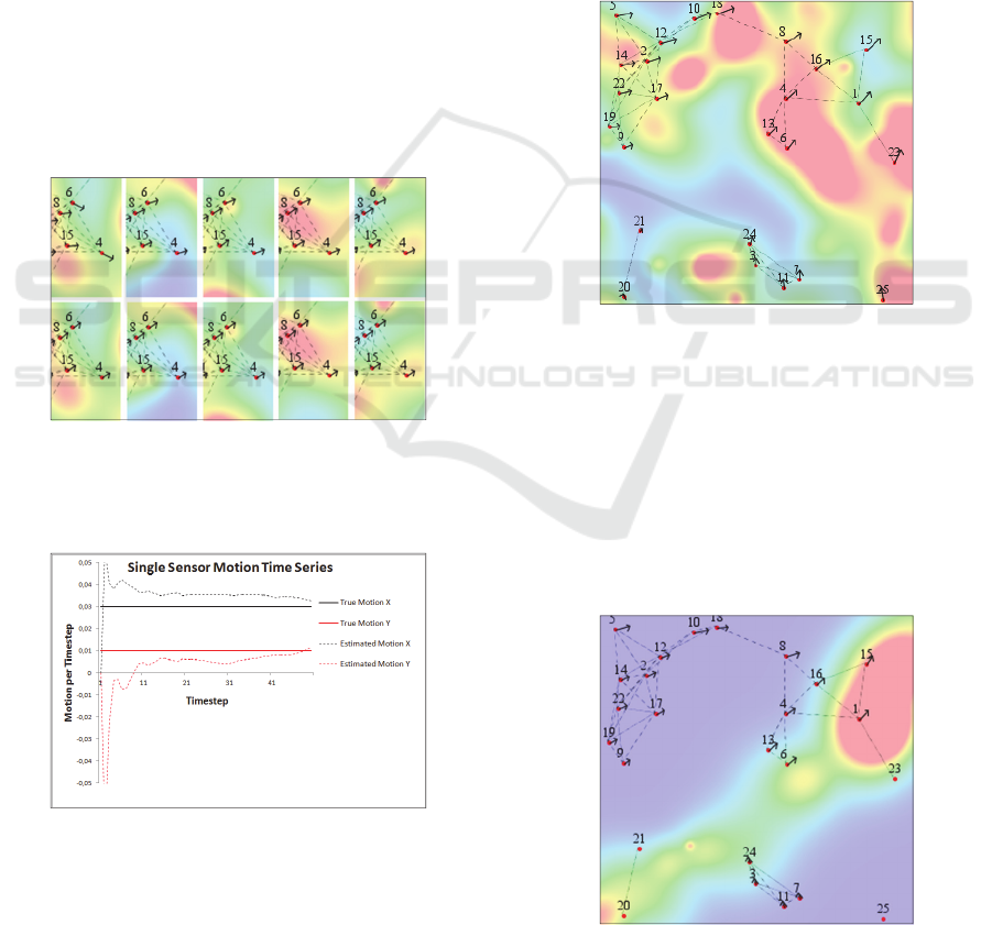
6.2.1 Constant Motion in Space and Time
In Figure 4, the difference between estimated (upper
row) and true motion (lower row) is displayed for a
particular experiment, some sensor nodes and
constant motion.
Figure 4: Constant Motion example. Estimated motion
time series (upper row) vs. true motion time series (lower
row). Temporal snapshots (columns) separated by 10
timesteps.
Figure 5: Constant Motion Example. Time series of
motion estimates (kalman state vector, dotted lines) of a
single sensor (sensor nr. 4 of Figure 4) vs. true motion
(solid lines).
At the beginning (first column), the motion
estimates are rather inaccurate. Over time, the
accuracy of the kalman motion estimates increases.
Figure 5 displays the whole time series of motion
estimates for a particular sensor node (node 4 of
Figure 4).
The inaccurate estimates eventually converge to
the true motion.
6.2.2 Spatially-varying Motion
As motion is estimated locally in the sensor
neighborhood, it is clear that the approach is able to
cope with locally spatially varying motion. In Figure
6, a snapshot of spatially inhomogeneous true
motion vectors is shown, where the vectors differ
with location.
Figure 6: Snapshot of a spatially inhomogeneous motion
field.
In Figure 7, the field of Figure 6 after 50
timesteps and estimated motion vectors are
displayed. Due to locality of motion estimation in
the sensor neighborhoods, the motion vectors adjust
to the local motion, e.g. there is a difference between
motion estimated in the upper left of the unit square
and the motion estimated in the lower part or upper
right part.
Figure 7: Snapshot of the experiment of Figure 6, 50
timesteps later and estimated motion vectors.
Decentralized Gradient-based Field Motion Estimation with a Wireless Sensor Network
21
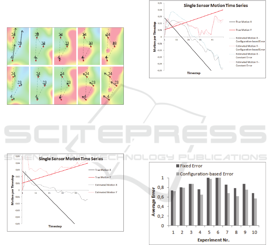
6.2.3 Dynamic Motion
In Figure 8, examples of an experiment with
dynamic motion is presented. Again, the upper row
shows estimated, the lower row true motion. The
true motion is manipulated each timestep. Again, the
motion estimates exhibit large errors at the
beginning and are refined over time. However, as
the kalman filter assumes constant motion, the
motion changes are only slowly adjusted and always
lag behind the true motion.
Figure 8: Dynamic Motion. Estimated motion times series
(upper row) vs. true motion time series (lower row).
Temporal snapshots (columns) separated by 10 timesteps.
This lag can also be recognized from the time
series of motion estimates of a single sensor (Figure).
Figure 9: Dynamic Motion Example. Time series of
motion estimates (i.e. kalman state vector, dotted lines) of
a single sensor (sensor nr. 23 from Figure 8) vs. true
motion (solid lines).
6.2.4 Fixed vs. Configuration-based Kalman
Measurement Noise
In another experiment, the methodology for error
estimation described in Section 4.4. is compared
with an assumed fixed kalman measurement error
variance, which is independent of the spatial
configuration. The simulations show, that the
proposed methodology indeed provides improved
motion estimates in most cases. Figure 10 shows an
example of the time series of motion estimates of a
single sensor for both methodologies. The
performance of the configuration-based error
estimation is, at most timesteps, improved (i.e.
estimated motion is closer to the true motion).
Figure 10: Comparison of the motion estimation
performance for a fixed kalman measurement error
variance vs. a configuration-based measurement error
variance and dynamic motion.
In Figure 11, the average motion estimation error
is displayed over all timesteps, sensor nodes and 10
different simulation runs. The error is calculated as
the norm of the vector difference between true and
estimated motion, normalized by the norm of true
motion.
Figure 11: Average overall error for a fixed kalman
measurement error variance (dark grey) and a
configuration-based measurement error variance (light
grey) for ten experiments.
The results show that the configuration-based
error provides an improvement in almost all
experiments. The magnitude of error depends on a
plethora of factors, mainly field properties.
Therefore, it is not further discussed here.
SENSORNETS 2016 - 5th International Conference on Sensor Networks
22

7 DISCUSSION & CONCLUSION
An approach for the decentralized estimation of the
motion of a spatio-temporal field with a WSN has
been presented. The performance of the algorithm
has been illustrated by examples of a simulated
dynamic field and sensor network. In the following,
possible extensions of the proposed algorithm are
discussed.
Sensor Network: Currently, stationary sensors and
time-synchronized sampling is assumed, since this is
considered the base case and eases the equations.
However, moving sensors monitoring spatio-
temporal fields, such as cars for measuring rainfall
(Fitzner et al., 2013); (Haberlandt and Sester, 2010),
exist and provide interesting possibilities for
extension. Further, the approach uses single-hop
communication and therefore assumes local
translational motion within the sensor neighborhood.
If motion is assumed to be constant over larger
neighborhoods, motion estimation accuracy could be
improved by multi-hop communication.
Accuracy of Gradient Constraint: Currently, the
accuracy of a gradient constraint is solely
determined by spatial configuration of the
neighborhood generating the constraint. However, it
is clear and already discussed in early work on
optical flow such as (Lucas et al., 1981) that field
properties such as the magnitude of the first or
second derivative are indicators of the accuracy.
Including these as well as weighting measures based
on spatial distance is planned for future extensions.
Kalman Filter: The kalman filter proposed in this
work comprises the motion vector only and
therefore, constant motion over time is assumed.
Possible motion changes are solely modeled by the
prediction error variance, which is larger zero and
hence, allows for state changes over time. A more
realistic assumption is motion change constancy that
could be implemented by adding motion change
variables to the kalman state. Further, the kalman
filter assumes white gaussian noise for both,
prediction and measurement, a requirement that has
to be tested in a real deployment of the algorithm. In
addition, the values for the kalman filter noise
parameters and have been set rather arbitrarily
based on a visual evaluation of the motion
estimation results. In future work, methods for
estimating these from the data will be investigated.
ACKNOWLEDGEMENTS
We gratefully acknowledge the financial support of
the German Research Foundation (DFG, SE645/8-
2).
REFERENCES
Bowler, N. E. H., Pierce, C. E., Seed, A., 2004.
Development of a precipitation nowcasting algorithm
based upon optical flow techniques. Journal of
Hydrology, vol. 288, no. 1-2, pp. 74–91.
Brink, J., Pebesma, E., 2014. Plume Tracking with a
Mobile Sensor Based on Incomplete and Imprecise
Information. Transactions in GIS, vol. 18, no. 5, pp.
740–766.
Das, J., Py, F., Maughan, T., O’Reilly, T., Messié, M.,
Ryan, J., Sukhatme, G.S., Rajan, K., 2012.
Coordinated sampling of dynamic oceanographic
features with underwater vehicles and drifters. The
International Journal of Robotics Research, vol. 31,
no. 5, pp. 626–646.
Duckham, M., 2012. Decentralized Spatial Computing:
Foundations of Geosensor Networks, Springer,
Heidelberg.
Fitzner, D., Sester, M., 2015. Estimation of precipitation
fields from 1-minute rain gauge time series –
comparison of spatial and spatio-temporal
interpolation methods. International Journal of
Geographical Information Science, vol. 29, nr. 9, pp.
1–26.
Fitzner, D., Sester, M., Haberlandt, U., Rabiei, E., 2013.
Rainfall Estimation with a Geosensor Network of Cars
Theoretical Considerations and First Results.
Photogrammetrie - Fernerkundung - Geoinformation,
vol. 2013, no. 2, pp. 93–103.
Fleet, D., Weiss, Y., 2006. Optical Flow Estimation, in:
Paragios, N., Chen, Y., Faugeras, O. (Eds.), Handbook
of Mathematical Models in Computer Vision. Springer
US, pp. 237–257.
Golub, G. H., Loan, C. F. V., 1996. Matrix Computations.
JHU Press.
Greg Welch, G. B., 2006. An Introduction to the Kalman
Filter, University of North Carolina, Technical Report
TR 95-041, July 24, 2006
Haberlandt, U., Sester, M., 2010. Areal rainfall estimation
using moving cars as rain gauges – a modelling study.
Hydrol. Earth Syst. Sci., vol. 14, no. 7, pp. 1139–1151.
Horn, B. K. P., Schunck, B. G., 1981. Determining optical
flow. Artificial Intelligence, vol. 17, no. 1-3, pp. 185–
203.
Huang, T. S., Hsu, Y. P., 1981. Image Sequence
Enhancement, in: Huang, P.T.S. (Ed.), Image
Sequence Analysis, Springer Series in Information
Sciences. Springer Berlin Heidelberg, pp. 289–309.
Jeong, M.-H., Duckham, M., Kealy, A., Miller, H. J.,
Peisker, A., 2014. Decentralized and coordinate-free
Decentralized Gradient-based Field Motion Estimation with a Wireless Sensor Network
23

computation of critical points and surface networks in
a discretized scalar field. International Journal of
Geographical Information Science, vol. 28, no. 1, pp.
1–21.
Kalman, R., 1960. A New Approach to Linear Filtering
and Prediction Problems. Transactions of the ASME –
Journal of Basic Engineering, vol. 82, no. 1, pp. 35–
45.
Langley, R. B., 1999. Dilution of precision. GPS world,
vol. 10, no. 5, 52–59.
Lucas, B. D., Kanade, T., others, 1981. An iterative image
registration technique with an application to stereo
vision., Proceedings of the 7
th
Intl. Joint Conference
on Artificial Intelligence, Vancouver, British
Columbia, pp. 674–679.
Särkkä, S., 2013. Bayesian Filtering and Smoothing.
Cambridge University Press.
Sester, M., 2009. Cooperative Boundary Detection in a
Geosensor Network using a SOM, Proceedings of the
International Cartographic Conference, Santiago,
Chile.
Tsai, H.-W., Chu, C.-P., Chen, T.-S., 2007. Mobile object
tracking in wireless sensor networks. Computer
Communications, vol. 30, no. 8, pp. 1811–1825.
Umer, M., Kulik, L., Tanin, E., 2010. Spatial interpolation
in wireless sensor networks: localized algorithms for
variogram modeling and Kriging. Geoinformatica, vol.
14, no. 1, pp. 101–134.
Watson, P. K., 1983. Kalman filtering as an alternative to
Ordinary Least Squares — Some theoretical
considerations and empirical results. Empirical
Economics, vol. 8, no. 2, pp. 71–85.
Zawadzki, I. I., 1973. Statistical Properties of Precipitation
Patterns. Journal of Applied Meteorology, vol. 12, pp.
459–472.
SENSORNETS 2016 - 5th International Conference on Sensor Networks
24
