
An Image Impairment Assessment Procedure using
the Saliency Map Technique
Hayato Teranaka
1
and Minoru Nakayama
2
1
Mechanical and Control Engineering, Tokyo Institute of Technology, O-okayama, Meguro-ku, Tokyo, 152–8552 Japan
2
Human System Science, Tokyo Institute of Technology, O-okayama, Meguro-ku, Tokyo, 152–8552 Japan
Keywords:
Image Quality Assessment, Image Impairment, Image Processing, Saliency Map, Subjective Evaluation.
Abstract:
An automated mechanical assessment procedure is required to evaluate image quality and impairment. This
paper proposes a procedure for image impairment assessment using visual attention, such as saliency maps
of the impaired images. To evaluate the performance of this image assessment procedure, an experiment was
conducted to study viewer’s subjective evaluations of impaired images, and the relationships between viewer’s
ratings and a previously developed set of values were then analyzed. Also, the limitations of the procedure
which was developed were discussed in order to improve assessment performance. The use of image features
and frequency-domain representation values for the test images was proposed.
1 INTRODUCTION
Image quality assessment is based on the human vi-
sion system, as the level of quality of an image is de-
fined by the subjective impressio of the viewer, who
compares various images by either viewing them di-
rectly or recalling them. As the cost to conduct an
evaluation of the subjective assessment of images is
high, various automated mechanical assessment pro-
cedures have been developed. Assessment is usually
based on certain features of images. Regarding this
approach, PSNR (Peak Signal to Noise Ratio) and
SSIM (Structural Similarity) are well known meth-
ods which are often used to assess image impairment
by comparing images to their originals (Tong et al.,
2006).
In order to develop an assessment procedure
which employs human visual processing, the mea-
surement of visual attention during the viewing of
objects by humans has often been considered (En-
gelke et al., 2011). Since visual attention affects
a viewer’s eye movements, the relationship between
image quality assessment and eye movement has
also been discussed (Engelke et al., 2011; Liu and
Heynderickx, 2011). One part of visual attention,
known as “bottom-up” information, can be used to
calculate various “saliency” (Itti et al., 1998; Guraya
et al., 2010; YuBing et al., 2011). Saliency informa-
tion, such as “saliency maps” is often used to pre-
dict the fixation area of eye movement (Itti, 2005).
The saliency of an image can often be a significant
source of information for image quality assessment
(Engelke et al., 2011; Liu and Heynderickx, 2011).
As techniques and metrics for image processing vary,
some hybrid visual attention assessment procedures
havebeen developed to assess image quality (Yu-Bing
et al., 2010; Jung, 2014).
Also, characteristics of image features such as
skewness and kurtosis can be metrics of image qual-
ity (Motoyoshi et al., 2007). A combination of image
features which includes information about frequency-
domain representation of the images can be a signifi-
cant resource for assessing image quality.
This paper proposes a procedure for image im-
pairment assessment using saliency maps to compare
impaired images with originals. This procedure is
a modification of the definition of PSNR calculation
procedure. Also, the limitations of the proposed pro-
cedure need to be discussed in order to improve as-
sessment performance.
2 IMAGE PROCESSING
PROCEDURES
2.1 Procedure using PSNR
A well known objective scale for image quality as-
sessment is PSNR (Peak Signal to Noise Ratio),
Teranaka, H. and Nakayama, M.
An Image Impairment Assessment Procedure using the Saliency Map Technique.
DOI: 10.5220/0005638600730078
In Proceedings of the 11th Joint Conference on Computer Vision, Imaging and Computer Graphics Theory and Applications (VISIGRAPP 2016) - Volume 4: VISAPP, pages 73-78
ISBN: 978-989-758-175-5
Copyright
c
2016 by SCITEPRESS – Science and Technology Publications, Lda. All rights reserved
73
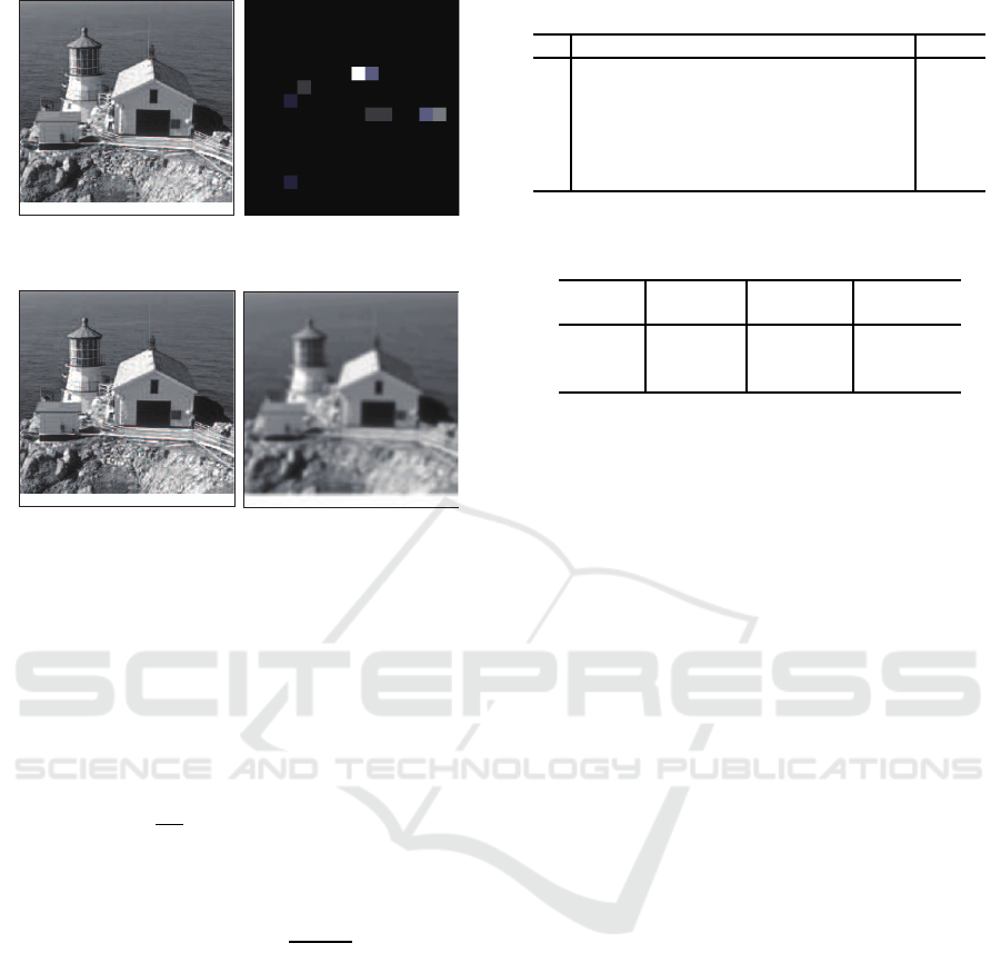
Figure 1: Original image (left) and Saliency map (right).
Figure 2: A pair of images presented for evaluation.
which measures the peak signal-to-noise ratio of im-
ages. The degree of image impairment can be calcu-
lated by summarizing the differences between each of
the pixels in the original and targeted images.
The following equation shows the mean square er-
ror of differences for each pixel of two monochrome
images I and K, where the image sizes of both are
m× n.
MSE =
1
mn
m
∑
i=1
n
∑
j=1
[I(i, j) − K(i, j)]
2
(1)
PSNR is defined using MSE.
PSNR = 10· log
10
MAX
I
2
MSE
(2)
Here, MAX
I
is the maximum brightness level of
the image. The value for an 8 bit monochrome image
is 255, for example. If two images are identical, the
PSNR is not defined since the MSE is zero. Regard-
ing the definition of PSNR, a high value of PSNR in-
dicates low image impairment. However, sometimes
this index does not reflect the viewer’ssubjective eval-
uation of image quality.
To improve this phenomenon, new procedures
such as SSIM (Structural Similarity) have been devel-
oped. They too have not yet been perfected, because
optional parameters still need to be set by evaluators.
Therefore, development of an index of image qual-
ity assessment which accurately reflects the viewer’s
subjective evaluations, has become necessary.
Table 1: Question items and means of ratings.
Question statement mean
1 Sharpness of the targeted image 3.0
2
Definition degree 2.9
3
Level of noise 2.7
4
Degree of expression in texture 2.8
5
Clearness of image content 3.3
6
Overall evaluation of image impairment 2.8
rating scale: 5: imperceptible – 1: very annoying
Table 2: Processing of impaired images using 3 filters.
GaussianBlur GaussianNoise ImpulseNoise
[radius: pixel] [STD: σ] [frequency: %]
Level 1 0.5 0.5 5
Level 2
1 10 10
Level 3
2 20 20
2.2 Saliency Map
Saliency is a feature of images which is used to re-
flect visual attention. This information indicates the
locality of an image.
Saliency is calculated using characteristics of im-
ages, such as color, brightness, and direction of edge,
which are summarized in a two-dimensional map
style that is known as a saliency map. The saliency
map of an image can be calculated using Saliency
ToolBox (Walter and Koch, 2006). An example of
a test image and a saliency map are shown in Figure
1.
2.3 Objective Scales using Saliency
Maps (OSSM)
Since a saliency map indicates a viewer’s visual atten-
tion, in addition to the features of an image, an objec-
tive scale for image assessment which uses saliency
maps has been developed. In this paper, a simple as-
sessment procedure using saliency maps (OSSM: ob-
jective scales using saliency maps) for image impair-
ment evaluation is proposed, and its limitations are
discussed.
The calculation procedure uses a comparison of
an original image K and its impaired image I, where
both are monochrome images (size m× n). A saliency
map for the impaired image is created using Saliency
ToolBox (Walter and Koch, 2006). The map informa-
tion (salmap(i, j)) is converted into the same size of
image (m × n). The differential squre values se(i, j)
between I and K are given by the squre of pixel dif-
ference such as equation 3.
se(i, j) = [I(i, j) − K(i, j)]
2
(3)
VISAPP 2016 - International Conference on Computer Vision Theory and Applications
74
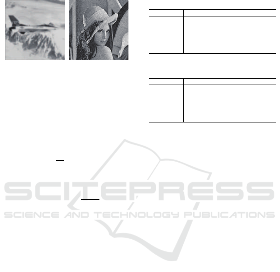
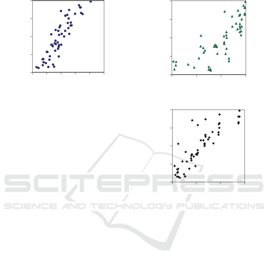
Figure 3: Examples of filtered images (Left: Airplane with
Gaussian Blur level 3; Right: Lena with Gaussian Noise
level 2).
A Napier constant of a value in the saliency map
e
salmap( i, j)
is weighted for square errors, se
sal
(i, j) is
considered the saliency.
se
sal
(i, j) = se(i, j) · e
salmap( i, j)
(4)
Mean square errors (MSE) of the overall image
are defined as a summation of the weighted square
errors equation 4.
MSE
sal
=
1
mn
m
∑
i=1
n
∑
j=1
se
sal
(i, j) (5)
The OSSM values are calculated using the follow-
ing equation 6 as well as 2 for PSNR.
OSSM = 10· log
10
MAX
I
2
MSE
sal
(6)
3 EVALUATION EXPERIMENT
3.1 Experimental Procedure
To evaluate the performance of OSSM, an image im-
pairment assessment test was conducted using a sub-
jective rating scale. This test employed six standard
images as test images. A pair of images, consisting
of an original and an impaired image, were displayed
on a 23 inch LCD monitor during an image evaluation
experiment, as shown in Figure 2. Participants rated a
targeted impaired image using the 6 question items in
Table 1 and a 5 point-scale, where 5: imperceptible,
4: perceptible, but not annoying, 3: slightly annoying,
2: annoying, and 1: very annoying.
The seven participants viewed and rated 54 im-
ages two times during two sessions, with a short break
in between.
3.2 Test Images
The target images were common monochrome test
pictures used in image processing. The image size
Table 3: Features of test images (originals).
Test image Mean Var skewness kurtosis
Airplane 179.1 2116 -1.347 3.771
Boat
144.0 1122 -1.493 5.152
Cameraman
119.2 3887 -0.736 2.090
Lena
123.0 2293 -0.078 2.174
Lighthouse
132.3 3383 0.653 2.768
Text
97.49 5177 1.091 2.858
Table 4: Features of frequency-domain representation val-
ues of test images analyzed using FFT.
Test image Mean Var skewness kurtosis
Airplane 4509 4509 4509 4509
Boat
3023 3023 3023 3023
Cameraman
4853 4853 4853 4853
Lena
5641 5641 5641 5641
Lighthouse
3855 3855 3855 3855
Text
97 5177 1.091 2.858
was 256 × 256 pixels, and the size displayed on a
PC was 768 × 768 pixels. Examples of images are
shown in Figure 3. Three levels of image processing
were provided, using image impairment filters such as
Gaussian blur, Gaussian noise and randomized noise,
as shown in Table 2. The total number of images
presented was 54 (6 images × 3 filters × 3 levels).
Statistics such as the mean, variance (Var), skewness
and kurtosis (Motoyoshi et al., 2007) of pixels in each
picture were calculated.
The image was processed and frequency-domain
representation components were extracted using FFT
(Fast Fourier Transforms). The same statistics were
also calculated for the features. The statistics for the
original images are summarized in Table 3, and ones
for the images which are processed using FFT are
summarized in Table 4.
Assessment metrics were calculated for every im-
age. Definitions of PSNR, SSIM and the proposed
procedure (OSSM) were calculated for each. The
metrics for PSNR and OSSM were computed in dB,
and a maximum of 1 was set for the SSIM metric.
4 EXPERIMENTAL RESULTS
The mean responses to 6 question items for all im-
paired test images are summarized in Table 1. The
means deviate around the middle level (slightly an-
noying) of the 5 point-scale. The responses to ques-
tion items were analyzed using factor analysis to de-
termine whether the responses consisted of any of the
factors. The results of factor analysis of viewer’s
responses show that they consist of a single factor.
Therefore, the overall averages of responses to the 6
questions are defined as subjective ratings.
An Image Impairment Assessment Procedure using the Saliency Map Technique
75
1
2
3
4
5
0 10 20 30 40 50
Subjective evaluation
Proposed method (OSSM) [dB]
r=0.89
Figure 4: Relationship between the proposed procedure
(OSSM) and subjective evaluation scores.
The relationship between the viewer’s rates and
automated evaluation metrics are summarized in Fig-
ures 4, 5, and 6 using scattergrams. The relation-
ship to the proposed procedure (OSSM) is indicated
in Figure 4, SSIM in Figure 5, and PSNR in Figure
6. There are strong correlations between the met-
rics of the automated evaluations and the subjective
ratings, and some deviations are observed in both re-
garding PSNR and SSIM. To evaluate these relation-
ships, correlation coefficients were calculated. The
coefficient for the proposed procedure (OSSM) is the
highest (r = 0.89) followed by SSIM (r = 0.80) and
PSNR (r = 0.86). Though the magnitudes of the cor-
relation coefficients are comparable among the three
procedures, the overall performance of the proposed
procedure (OSSM) is better than that of the other two.
Deviations in rating test images may influence the as-
sessment performance, and these differences are ana-
lyzed in the discussion section, in order to emphasize
the benefits of the proposed procedure (OSSM).
5 DISCUSSION
5.1 Assessment Differences among Test
Images
Image quality assessment may depend on the features
of the images, and the relationships between viewer’s
responses and the above-mentioned features. These
were evaluated for each set of test images using a
correlation coefficient, and are summarized in Table
5. Regarding the assessment metric definitions, high
coefficients for PSNR and the proposed procedure
(OSSM) were observed. In the results, most coeffi-
cients for OSSM and PSNR are high, except for one
image set (Text), and are higher than the coefficients
for SSIM.
1
2
3
4
5
0.4 0.6 0.8 1
SSIM [dB]
Subjective evaluation
r=0.80
Figure 5: Relationship between SSIM procedure and sub-
jective evaluation scores.
1
2
3
4
5
20 30 40 50
PSNR [dB]
Subjective evaluation
r=0.86
Figure 6: Relationship between PSNR procedure and sub-
jective evaluation scores.
In addition to calculating correlation coefficients,
the prediction accuracy of the ratings is discussed.
Linear regression functions were calculated for each
evaluation procedure, in order to measure the devia-
tions in scattergrams between the results of mechan-
ical assessments and viewer’s ratings. To evaluate
the degree of fitness using linear regression predic-
tion, RMSE (root mean squared error) was calculated
by comparing the prediction values with the functions
and viewer’s assessment ratings. The results are sum-
marized on the right hand side of Table 5. Means
of RMSE for images are also comparable between
OSSM and PSNR, and are smaller than the means for
SSIM. In particular, the RMSE means using OSSM
are slightly smaller than the means for PSNR, and are
indicated in Table 5 using underlining. These results
suggest that OSSM can produce a better index of im-
age impairment. Since assessment performance de-
pends on the test images, some specific features of
images may contribute to the index.
In Table 5, both coefficients and means of RMSE
for test image ”Text” show significantly different val-
ues when compared to other test images. A detailed
VISAPP 2016 - International Conference on Computer Vision Theory and Applications
76
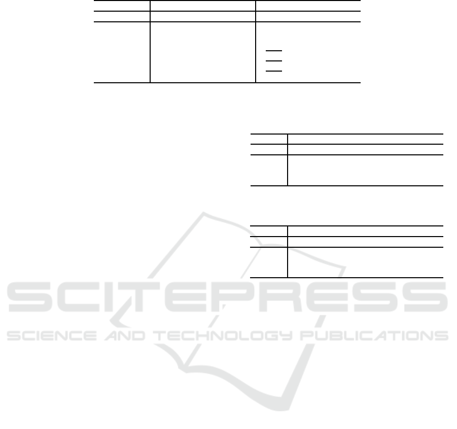
Table 5: Relationships between automated and viewer’s evaluations of all test images.
r RMSE
Test image OSSM SSIM PSNR OSSM SSIM PSNR
Airplane 0.96 0.75 0.97 0.79 3.87 0.61
Boat
0.96 0.81 0.97 0.68 2.84 0.51
Cameraman
0.98 0.78 0.97 0.39 3.84 0.53
Lena
0.98 0.78 0.98 0.29 2.32 0.32
Lighthouse
0.98 0.94 0.97 0.47 1.07 0.55
Text
0.81 0.80 0.82 2.91 3.08 2.79
OSSM: Objective scale using Saliency Map
analysis was conducted in order to reveal the cause of
this difference.
5.2 Relationship with Features of
Images
The features of images, consisting of the means, vari-
ances, skewness and kurtosis of both the pixel data
of the images and the frequency-domain representa-
tion values of FFT images, were employed to extract
the features. To examine the relationship between the
above mentioned RMSE and these features, correla-
tion coefficients were calculated and summarized in
Tables 6 and 7. Most of the relationship coefficients
of the FFT images are significant. The absolute coef-
ficients of skewness and kurtosis for FFT images are
higher than 0.7, and the significant contributions of
skewness and kurtosis are confirmed. These indices
are concerned with the assessment of image quality
in the previous study (Motoyoshi et al., 2007), and
the results of this research support the previous work.
As was mentioned above, image impairment as-
sessment performance depends on the test images.
The feature differences of the images were analyzed
using the statistics of the images, in particular using
the FFT images. Regarding the statistics in Tables
3 and 4, the proposed procedure (OSSM) shows the
best performance when the skewness of the FFT im-
ages is 185–215, and the kurtosis of the FFT images
is 42000–51000. However, PSNR shows a higher
level of performance, with the exception of the above-
mentioned condition.
6 CONCLUSION
This paper has proposed a procedure for image im-
pairment assessment using saliency maps to compare
impaired images to their originals. The performance
of this method was comparedto two conventionalpro-
cedures.
To evaluate image assessment performance, an
experiment was conducted using viewer’s subjective
Table 6: Coefficients between RMSE and features of im-
ages.
Features of images
proc. Mean Var skewness kurtosis
OSSM -0.479 0.654 0.542 0.038
SSIM
0.219 0.025 -0.537 0.116
PSNR
-0.571 0.743 0.623 -0.078
Table 7: Coefficients between RMSE and features of FFT
images.
Features of FFT images
proc. Mean Var skewness kurtosis
OSSM 0.357 -0.338 -0.728 -0.704
SSIM
0.217 0.425 -0.068 -0.070
PSNR
0.416 -0.433 -0.808 -0.787
evaluations of impaired images. The correlation coef-
ficients for the evaluated scores of the proposed pro-
cedure (OSSM) are the highest all of the three of the
procedures. RMSEs between viewer’s ratings and the
predicted linear regression values were calculated as
an index of fitness, and assessment performance was
then compared. For some test images, the OSSM
RMSEs are smaller than those for the other two pro-
cedures. The limitations of the proposed procedure
were discussed in regards to the deviations of correla-
tion coefficients and RMSEs across test images.
The improvement of image assessment perfor-
mance and the development of an image quality as-
sessment procedure for single images will be subjects
of our further study.
REFERENCES
Engelke, U., Kaprykowsky, H., Zepernick, H., and Jdjiki-
Nya., P. (2011). Visual attention in quality assessment.
IEEE Signal Processing Magazine, 50.
Guraya, F. F. E., Cheikh, F. A., Tr´emeau, A., Tong, Y.,
and Konik, H. (2010). Predictive Saliency Maps for
Surveillance Videos. In Proc. of 2010 Ninth Inter-
national Symposium on Distributed Computing and
Applications to Business, Engineering and Science,
pages 508–513.
Itti, L. (2005). Quantifying the contribution of low-level
An Image Impairment Assessment Procedure using the Saliency Map Technique
77

saliency to human eye movements in dynamic scenes.
Visual Cognition, 12(6):1093–1123.
Itti, L., Koch, C., and Niebur, E. (1998). A model of
saliency-based visual attention for rapid scene anal-
ysis. IEEE Trans. Pattern Analysis and Machine In-
telligence, 20(11):1254–1259.
Jung, C. (2014). Hybrid integration of visual attention
model into image quality metric. IEICE Trans. INF.
& SYST., E97-D(11):2971–2973.
Liu, H. and Heynderickx, I. (2011). Visual attention in
objective image quality assessment: Based on eye-
tracking data. IEEE Trans. Circuits and Systems for
Video Technology, 21(7):971–982.
Motoyoshi, I., Nishida, S., Sharan, L., and Adelson, E. H.
(2007). Image statistics and the perception of surface
qualities. Nature, 447:206–209.
Tong, Y.-B., Chang, Q., and Zhang, Q.-S. (2006). Image
Quality Assessing by using NN and SVM. In Proc. of
Fifth International Conference on Machine Learning
and Cybernetics, pages 3987–3990.
Walter, D. and Koch, C. (2006). Modeling at-
tention to salient proto-objects. Neural Net-
works, 19:1395–1407.
Software available at
http://www.saliencytoolbox.net
.
Yu-Bing, T., Konik, H., Cheikh, F. A., and Tremeau,
A. (2010). Full reference image quality assessment
based on saliency map analysis. International Jounal
of Imaging Science and Technology, 54(3):030503–
030514.
YuBing, T., Cheikh, F. A., Guraya, F. F. E., Konik, H., and
Tr´emeau, A. (2011). A spatiotemporal saliency model
for video surveillance. Journal of Cognitive Comput-
ing, 3(1):241–263.
VISAPP 2016 - International Conference on Computer Vision Theory and Applications
78
